Execute this notebook: Download locally

Node representations with GraphWave

This demo features the algorithm GraphWave published in “Learning Structural Node Embeddings via Diffusion Wavelets” [https://arxiv.org/pdf/1710.10321.pdf]. GraphWave embeds the structural features of a node in a dense embeddings. We will demonstrate the use of GraphWave on a barbell graph demonstrating that structurally equivalent nodes have similar embeddings.

First, we load the required libraries.

import networkx as nx
from stellargraph.mapper import GraphWaveGenerator
from stellargraph import StellarGraph
from sklearn.decomposition import PCA
import numpy as np
from matplotlib import pyplot as plt
from scipy.sparse.linalg import eigs
import tensorflow as tf
from tensorflow.keras import backend as K

Graph construction

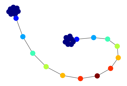
Next, we construct the barbell graph, shown below. It consists of 2 fully connected graphs (at the ‘ends’ of the graph) connected by a chain of nodes. All nodes in the fully connected ends are structurally equivalent, as are the opposite nodes in the chain. A good structural embedding algorithm should embed equivalent nodes close together in the embedding space.

m1 = 9
m2 = 11
gnx = nx.barbell_graph(m1=m1, m2=m2)

classes = [0,] * len(gnx.nodes)
# number of nodes with a non-zero class (the path, plus the nodes it connects to on either end)
nonzero = m2 + 2
# count up to the halfway point (rounded up)
first = range(1, (nonzero + 1) // 2 + 1)
# and down for the rest
second = reversed(range(1, nonzero - len(first) + 1))
classes[m1 - 1 : (m1 + m2) + 1] = list(first) + list(second)

nx.draw(gnx, node_color=classes, cmap="jet")

GraphWave embedding calculation

Now, we’re ready to calculate the GraphWave embeddings. We need to specify some information about the approximation to use:

• an iterable of wavelet scales to use. This is a graph and task dependent hyperparameter. Larger scales extract larger scale features and smaller scales extract more local structural features. Experiment with different values.

• the sample_points at which to sample the characteristic function. This should be of the form sample_points=np.linspace(0, max_val, number_of_samples). The best value depends on the graph.

• the degree of Chebyshev poly

The dimension of the embeddings are 2 * len(scales) * len(sample_points)

G = StellarGraph.from_networkx(gnx)
sample_points = np.linspace(0, 100, 50).astype(np.float32)
degree = 20
scales = [5, 10]

generator = GraphWaveGenerator(G, scales=scales, degree=degree)

embeddings_dataset = generator.flow(
    node_ids=G.nodes(), sample_points=sample_points, batch_size=1, repeat=False
)

embeddings = [x.numpy() for x in embeddings_dataset]

Visualisation

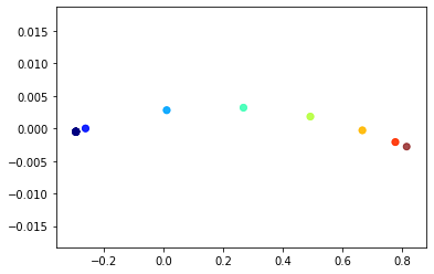
The nodes are coloured by their structural role, e.g. in the fully connected sections, first node in the chain, second node in the chain etc. We can see that all nodes of the same colour completely overlap in this visualisation, indicating that structurally equivalent nodes are very close in the embedding space.

The plot here doesn’t exactly match the one in the paper, which we think is because the details of approximating the wavelet diffusion differ, the paper uses pygsp to calculate the Chebyshev coefficient while StellarGraph uses numpy to calculate the coefficients. Some brief experiments have shown that the numpy Chebyshev coefficients are more accurate than the pygsp coefficients.

trans_emb = PCA(n_components=2).fit_transform(np.vstack(embeddings))

plt.scatter(
    trans_emb[:, 0], trans_emb[:, 1], c=classes, cmap="jet", alpha=0.7,
)
plt.show()

Execute this notebook: Download locally