Execute this notebook:
Download locally
Unsupervised graph classification/representation learning via distances
This demo demonstrated training a graph classification model without supervision. This model could be used to compute embedding vectors or representations for graphs.
The algorithm uses a ground-truth distance between graphs as a metric to train against, by embedding pairs of graphs simultaneously and combining the resulting embedding vectors to match the distance.
It is inspired by UGraphEmb[1].
[1]: Y. Bai et al., “Unsupervised Inductive Graph-Level Representation Learning via Graph-Graph Proximity,” arXiv:1904.01098 [cs, stat], Jun. 2019.
[3]:
import stellargraph as sg
import pandas as pd
import numpy as np
import networkx as nx
import tensorflow as tf
from tensorflow import keras

from IPython.display import display, HTML
Dataset
The PROTEINS dataset consists of about one thousand graphs, with binary labels 1 or 2.
[4]:
dataset = sg.datasets.PROTEINS()
display(HTML(dataset.description))
graphs, graph_labels = dataset.load()
[5]:
graph_labels.value_counts().to_frame()
[5]:
| label | |
|---|---|
| 1 | 663 |
| 2 | 450 |
The graphs value consists of many StellarGraph instances:
[6]:
print(graphs[0].info())
StellarGraph: Undirected multigraph
 Nodes: 42, Edges: 162

 Node types:
  default: [42]
    Features: float32 vector, length 4
    Edge types: default-default->default

 Edge types:
    default-default->default: [162]
        Weights: all 1 (default)
        Features: none
Summary statistics of the sizes of the graphs:
[7]:
summary = pd.DataFrame(
    [(g.number_of_nodes(), g.number_of_edges()) for g in graphs],
    columns=["nodes", "edges"],
)
summary.describe().round(1)
[7]:
| nodes | edges | |
|---|---|---|
| count | 1113.0 | 1113.0 |
| mean | 39.1 | 145.6 |
| std | 45.8 | 169.3 |
| min | 4.0 | 10.0 |
| 25% | 15.0 | 56.0 |
| 50% | 26.0 | 98.0 |
| 75% | 45.0 | 174.0 |
| max | 620.0 | 2098.0 |
Create the model
[8]:
generator = sg.mapper.PaddedGraphGenerator(graphs)
[9]:
gc_model = sg.layer.GCNSupervisedGraphClassification(
    [64, 32], ["relu", "relu"], generator, pool_all_layers=True
)
[10]:
inp1, out1 = gc_model.in_out_tensors()
inp2, out2 = gc_model.in_out_tensors()

vec_distance = tf.norm(out1 - out2, axis=1)
[11]:
pair_model = keras.Model(inp1 + inp2, vec_distance)
embedding_model = keras.Model(inp1, out1)
Train the model
The model is trained on 100 random pairs of graphs, along with the ground-truth distance between them.
Similarity measure
This method can use any notion of distance or similarity between two graphs. In this case, we use something efficient, but not particularly accurate: the distance between the spectrum (or eigenvalues) of the Laplacian matrix of the graphs.
Other options include graph edit distance and minimum common subgraph, but these are NP-hard to compute and are too slow for this demonstration.
[12]:
def graph_distance(graph1, graph2):
    spec1 = nx.laplacian_spectrum(graph1.to_networkx(feature_attr=None))
    spec2 = nx.laplacian_spectrum(graph2.to_networkx(feature_attr=None))
    k = min(len(spec1), len(spec2))
    return np.linalg.norm(spec1[:k] - spec2[:k])
Training examples
[13]:
graph_idx = np.random.RandomState(0).randint(len(graphs), size=(100, 2))
[14]:
targets = [graph_distance(graphs[left], graphs[right]) for left, right in graph_idx]
[15]:
train_gen = generator.flow(graph_idx, batch_size=10, targets=targets)
Training procedure
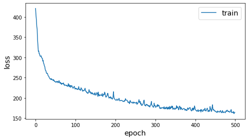
[16]:
pair_model.compile(keras.optimizers.Adam(1e-2), loss="mse")
[17]:
%%time
history = pair_model.fit(train_gen, epochs=500, verbose=0)
sg.utils.plot_history(history)
  ['...']
CPU times: user 3min 30s, sys: 1min 40s, total: 5min 11s
Wall time: 1min 17s

Compute embeddings
[18]:
embeddings = embedding_model.predict(generator.flow(graphs))
Downstream tasks
Now that we’ve computed some embedding vectors in an unsupervised fashion, we can use them for other supervised, semi-supervised and unsupervised tasks.
Supervised graph classification
We can use the embedding vectors to perform logistic regression classification, using the labels.
[19]:
from sklearn.linear_model import LogisticRegression
from sklearn import model_selection
[20]:
train_labels, test_labels = model_selection.train_test_split(
    graph_labels, train_size=0.1, test_size=None, stratify=graph_labels
)

test_embeddings = embeddings[test_labels.index - 1]
train_embeddings = embeddings[train_labels.index - 1]

lr = LogisticRegression(multi_class="auto", solver="lbfgs")
lr.fit(train_embeddings, train_labels)

y_pred = lr.predict(test_embeddings)
gcn_acc = (y_pred == test_labels).mean()
print(f"Test classification accuracy: {gcn_acc}")
Test classification accuracy: 0.6846307385229541
Confusion matrix
[21]:
pd.crosstab(test_labels, y_pred, rownames=["true"], colnames=["predicted"])
[21]:
| predicted | 1 | 2 |
|---|---|---|
| true | ||
| 1 | 506 | 91 |
| 2 | 225 | 180 |
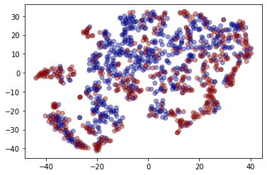
Visualising embeddings
We can also get a qualitative measure of the embeddings, using dimensionality reduction.
[22]:
from sklearn.manifold import TSNE

tsne = TSNE(2)
two_d = tsne.fit_transform(embeddings)
[23]:
from matplotlib import pyplot as plt

plt.scatter(two_d[:, 0], two_d[:, 1], c=graph_labels.cat.codes, cmap="jet", alpha=0.4)
[23]:
<matplotlib.collections.PathCollection at 0x163db1a20>

Conclusion
This demo demonstrated training a graph classification model without supervision. This model could be used to compute embedding vectors or representations for graphs.
The algorithm works with three components:
a ground truth distance or similarity between two graphs such as graph edit distance, or, in this case, Laplacian spectrum distance (for efficiency)
a model that encodes graphs into embedding vectors
a data generator that yields pairs of graphs and the corresponding ground truth distance
This model is inspired by UGraphEmb[1].
Execute this notebook:
Download locally
