Execute this notebook:
![]()
![]() Download locally
Download locally
Node classification with GraphSAGE
Import stellargraph:
[3]:
import networkx as nx
import pandas as pd
import os

import stellargraph as sg
from stellargraph.mapper import GraphSAGENodeGenerator
from stellargraph.layer import GraphSAGE

from tensorflow.keras import layers, optimizers, losses, metrics, Model
from sklearn import preprocessing, feature_extraction, model_selection
from stellargraph import datasets
from IPython.display import display, HTML
import matplotlib.pyplot as plt
%matplotlib inline
Loading the CORA network
(See the “Loading from Pandas” demo for details on how data can be loaded.)
[4]:
dataset = datasets.Cora()
display(HTML(dataset.description))
G, node_subjects = dataset.load()
[5]:
print(G.info())
StellarGraph: Undirected multigraph
 Nodes: 2708, Edges: 5429

 Node types:
  paper: [2708]
    Edge types: paper-cites->paper

 Edge types:
    paper-cites->paper: [5429]
We aim to train a graph-ML model that will predict the “subject” attribute on the nodes. These subjects are one of 7 categories:
[6]:
set(node_subjects)
[6]:
{'Case_Based',
 'Genetic_Algorithms',
 'Neural_Networks',
 'Probabilistic_Methods',
 'Reinforcement_Learning',
 'Rule_Learning',
 'Theory'}
Splitting the data
For machine learning we want to take a subset of the nodes for training, and use the rest for testing. We’ll use scikit-learn again to do this
[7]:
train_subjects, test_subjects = model_selection.train_test_split(
    node_subjects, train_size=0.1, test_size=None, stratify=node_subjects
)
Note using stratified sampling gives the following counts:
[8]:
from collections import Counter

Counter(train_subjects)
[8]:
Counter({'Probabilistic_Methods': 42,
         'Genetic_Algorithms': 42,
         'Reinforcement_Learning': 22,
         'Rule_Learning': 18,
         'Neural_Networks': 81,
         'Case_Based': 30,
         'Theory': 35})
The training set has class imbalance that might need to be compensated, e.g., via using a weighted cross-entropy loss in model training, with class weights inversely proportional to class support. However, we will ignore the class imbalance in this example, for simplicity.
Converting to numeric arrays
For our categorical target, we will use one-hot vectors that will be fed into a soft-max Keras layer during training. To do this conversion …
[9]:
target_encoding = preprocessing.LabelBinarizer()

train_targets = target_encoding.fit_transform(train_subjects)
test_targets = target_encoding.transform(test_subjects)
We now do the same for the node attributes we want to use to predict the subject. These are the feature vectors that the Keras model will use as input. The CORA dataset contains attributes ‘w_x’ that correspond to words found in that publication. If a word occurs more than once in a publication the relevant attribute will be set to one, otherwise it will be zero.
Creating the GraphSAGE model in Keras
To feed data from the graph to the Keras model we need a data generator that feeds data from the graph to the model. The generators are specialized to the model and the learning task so we choose the GraphSAGENodeGenerator as we are predicting node attributes with a GraphSAGE model.
We need two other parameters, the batch_size to use for training and the number of nodes to sample at each level of the model. Here we choose a two-level model with 10 nodes sampled in the first layer, and 5 in the second.
[10]:
batch_size = 50
num_samples = [10, 5]
A GraphSAGENodeGenerator object is required to send the node features in sampled subgraphs to Keras
[11]:
generator = GraphSAGENodeGenerator(G, batch_size, num_samples)
Using the generator.flow() method, we can create iterators over nodes that should be used to train, validate, or evaluate the model. For training we use only the training nodes returned from our splitter and the target values. The shuffle=True argument is given to the flow method to improve training.
[12]:
train_gen = generator.flow(train_subjects.index, train_targets, shuffle=True)
Now we can specify our machine learning model, we need a few more parameters for this:
the
layer_sizesis a list of hidden feature sizes of each layer in the model. In this example we use 32-dimensional hidden node features at each layer.The
biasanddropoutare internal parameters of the model.
[13]:
graphsage_model = GraphSAGE(
    layer_sizes=[32, 32], generator=generator, bias=True, dropout=0.5,
)
Now we create a model to predict the 7 categories using Keras softmax layers.
[14]:
x_inp, x_out = graphsage_model.in_out_tensors()
prediction = layers.Dense(units=train_targets.shape[1], activation="softmax")(x_out)
Training the model
Now let’s create the actual Keras model with the graph inputs x_inp provided by the graph_model and outputs being the predictions from the softmax layer
[15]:
model = Model(inputs=x_inp, outputs=prediction)
model.compile(
    optimizer=optimizers.Adam(lr=0.005),
    loss=losses.categorical_crossentropy,
    metrics=["acc"],
)
Train the model, keeping track of its loss and accuracy on the training set, and its generalisation performance on the test set (we need to create another generator over the test data for this)
[16]:
test_gen = generator.flow(test_subjects.index, test_targets)
[17]:
history = model.fit(
    train_gen, epochs=20, validation_data=test_gen, verbose=2, shuffle=False
)
Epoch 1/20
6/6 - 2s - loss: 1.8488 - acc: 0.3037 - val_loss: 1.6904 - val_acc: 0.3794
Epoch 2/20
6/6 - 2s - loss: 1.6272 - acc: 0.4852 - val_loss: 1.5230 - val_acc: 0.5349
Epoch 3/20
6/6 - 2s - loss: 1.4474 - acc: 0.6333 - val_loss: 1.3641 - val_acc: 0.6829
Epoch 4/20
6/6 - 2s - loss: 1.2771 - acc: 0.7630 - val_loss: 1.2483 - val_acc: 0.7186
Epoch 5/20
6/6 - 2s - loss: 1.1698 - acc: 0.8444 - val_loss: 1.1501 - val_acc: 0.7498
Epoch 6/20
6/6 - 2s - loss: 1.0364 - acc: 0.9000 - val_loss: 1.0619 - val_acc: 0.7756
Epoch 7/20
6/6 - 2s - loss: 0.9260 - acc: 0.8963 - val_loss: 0.9960 - val_acc: 0.7896
Epoch 8/20
6/6 - 2s - loss: 0.8232 - acc: 0.9000 - val_loss: 0.9372 - val_acc: 0.7986
Epoch 9/20
6/6 - 2s - loss: 0.7396 - acc: 0.9481 - val_loss: 0.8897 - val_acc: 0.8056
Epoch 10/20
6/6 - 2s - loss: 0.6708 - acc: 0.9630 - val_loss: 0.8496 - val_acc: 0.8056
Epoch 11/20
6/6 - 2s - loss: 0.5816 - acc: 0.9667 - val_loss: 0.8084 - val_acc: 0.8162
Epoch 12/20
6/6 - 2s - loss: 0.5232 - acc: 0.9852 - val_loss: 0.7748 - val_acc: 0.8175
Epoch 13/20
6/6 - 2s - loss: 0.4801 - acc: 0.9778 - val_loss: 0.7515 - val_acc: 0.8154
Epoch 14/20
6/6 - 2s - loss: 0.4383 - acc: 0.9852 - val_loss: 0.7452 - val_acc: 0.8097
Epoch 15/20
6/6 - 2s - loss: 0.4116 - acc: 0.9778 - val_loss: 0.7161 - val_acc: 0.8187
Epoch 16/20
6/6 - 2s - loss: 0.3584 - acc: 0.9889 - val_loss: 0.7039 - val_acc: 0.8187
Epoch 17/20
6/6 - 2s - loss: 0.3559 - acc: 0.9815 - val_loss: 0.6767 - val_acc: 0.8240
Epoch 18/20
6/6 - 2s - loss: 0.3104 - acc: 0.9889 - val_loss: 0.6849 - val_acc: 0.8146
Epoch 19/20
6/6 - 2s - loss: 0.2925 - acc: 0.9815 - val_loss: 0.6698 - val_acc: 0.8162
Epoch 20/20
6/6 - 2s - loss: 0.2690 - acc: 0.9852 - val_loss: 0.6559 - val_acc: 0.8199
[18]:
sg.utils.plot_history(history)
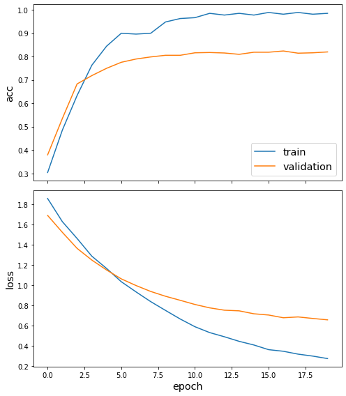
Now we have trained the model we can evaluate on the test set.
[19]:
test_metrics = model.evaluate(test_gen)
print("\nTest Set Metrics:")
for name, val in zip(model.metrics_names, test_metrics):
    print("\t{}: {:0.4f}".format(name, val))
Test Set Metrics:
        loss: 0.6601
        acc: 0.8228
Making predictions with the model
Now let’s get the predictions themselves for all nodes using another node iterator:
[20]:
all_nodes = node_subjects.index
all_mapper = generator.flow(all_nodes)
all_predictions = model.predict(all_mapper)
These predictions will be the output of the softmax layer, so to get final categories we’ll use the inverse_transform method of our target attribute specification to turn these values back to the original categories
[21]:
node_predictions = target_encoding.inverse_transform(all_predictions)
Let’s have a look at a few:
[22]:
df = pd.DataFrame({"Predicted": node_predictions, "True": node_subjects})
df.head(10)
[22]:
| Predicted | True | |
|---|---|---|
| 31336 | Neural_Networks | Neural_Networks |
| 1061127 | Rule_Learning | Rule_Learning |
| 1106406 | Reinforcement_Learning | Reinforcement_Learning |
| 13195 | Reinforcement_Learning | Reinforcement_Learning |
| 37879 | Probabilistic_Methods | Probabilistic_Methods |
| 1126012 | Reinforcement_Learning | Probabilistic_Methods |
| 1107140 | Reinforcement_Learning | Theory |
| 1102850 | Neural_Networks | Neural_Networks |
| 31349 | Neural_Networks | Neural_Networks |
| 1106418 | Theory | Theory |
Create a NetworkX graph to save it as GraphML, e.g. for visualisation in Gephi. This adds the predictions to the graph before saving too.
[23]:
Gnx = G.to_networkx(feature_attr=None)
[24]:
for nid, pred, true in zip(df.index, df["Predicted"], df["True"]):
    Gnx.nodes[nid]["subject"] = true
    Gnx.nodes[nid]["PREDICTED_subject"] = pred.split("=")[-1]
Also add isTrain and isCorrect node attributes:
[25]:
for nid in train_subjects.index:
    Gnx.nodes[nid]["isTrain"] = True

for nid in test_subjects.index:
    Gnx.nodes[nid]["isTrain"] = False
[26]:
for nid in Gnx.nodes():
    Gnx.nodes[nid]["isCorrect"] = (
        Gnx.nodes[nid]["subject"] == Gnx.nodes[nid]["PREDICTED_subject"]
    )
Save in GraphML format
[27]:
pred_fname = "pred_n={}.graphml".format(num_samples)
nx.write_graphml(Gnx, os.path.join(dataset.data_directory, pred_fname))
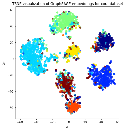
Node embeddings
Evaluate node embeddings as activations of the output of GraphSAGE layer stack, and visualise them, coloring nodes by their subject label.
The GraphSAGE embeddings are the output of the GraphSAGE layers, namely the x_out variable. Let’s create a new model with the same inputs as we used previously x_inp but now the output is the embeddings rather than the predicted class. Additionally note that the weights trained previously are kept in the new model.
[28]:
embedding_model = Model(inputs=x_inp, outputs=x_out)
[29]:
emb = embedding_model.predict(all_mapper)
emb.shape
[29]:
(2708, 32)
Project the embeddings to 2d using either TSNE or PCA transform, and visualise, coloring nodes by their subject label
[30]:
from sklearn.decomposition import PCA
from sklearn.manifold import TSNE
import pandas as pd
import numpy as np
[31]:
X = emb
y = np.argmax(target_encoding.transform(node_subjects), axis=1)
[32]:
if X.shape[1] > 2:
    transform = TSNE  # PCA

    trans = transform(n_components=2)
    emb_transformed = pd.DataFrame(trans.fit_transform(X), index=node_subjects.index)
    emb_transformed["label"] = y
else:
    emb_transformed = pd.DataFrame(X, index=node_subjects.index)
    emb_transformed = emb_transformed.rename(columns={"0": 0, "1": 1})
    emb_transformed["label"] = y
[33]:
alpha = 0.7

fig, ax = plt.subplots(figsize=(7, 7))
ax.scatter(
    emb_transformed[0],
    emb_transformed[1],
    c=emb_transformed["label"].astype("category"),
    cmap="jet",
    alpha=alpha,
)
ax.set(aspect="equal", xlabel="$X_1$", ylabel="$X_2$")
plt.title(
    "{} visualization of GraphSAGE embeddings for cora dataset".format(transform.__name__)
)
plt.show()
Execute this notebook:
![]()
![]() Download locally
Download locally
