Execute this notebook:
![]()
![]() Download locally
Download locally
Node classification with Graph ATtention Network (GAT)
Import NetworkX and stellar:
[3]:
import networkx as nx
import pandas as pd
import os

import stellargraph as sg
from stellargraph.mapper import FullBatchNodeGenerator
from stellargraph.layer import GAT

from tensorflow.keras import layers, optimizers, losses, metrics, Model
from sklearn import preprocessing, feature_extraction, model_selection
from stellargraph import datasets
from IPython.display import display, HTML
import matplotlib.pyplot as plt
%matplotlib inline
Loading the CORA network
(See the “Loading from Pandas” demo for details on how data can be loaded.)
[4]:
dataset = datasets.Cora()
display(HTML(dataset.description))
G, node_subjects = dataset.load()
[5]:
print(G.info())
StellarGraph: Undirected multigraph
 Nodes: 2708, Edges: 5429

 Node types:
  paper: [2708]
    Edge types: paper-cites->paper

 Edge types:
    paper-cites->paper: [5429]
We aim to train a graph-ML model that will predict the “subject” attribute on the nodes. These subjects are one of 7 categories:
[6]:
set(node_subjects)
[6]:
{'Case_Based',
 'Genetic_Algorithms',
 'Neural_Networks',
 'Probabilistic_Methods',
 'Reinforcement_Learning',
 'Rule_Learning',
 'Theory'}
Splitting the data
For machine learning we want to take a subset of the nodes for training, and use the rest for validation and testing. We’ll use scikit-learn again to do this.
Here we’re taking 140 node labels for training, 500 for validation, and the rest for testing.
[7]:
train_subjects, test_subjects = model_selection.train_test_split(
    node_subjects, train_size=140, test_size=None, stratify=node_subjects
)
val_subjects, test_subjects = model_selection.train_test_split(
    test_subjects, train_size=500, test_size=None, stratify=test_subjects
)
Note using stratified sampling gives the following counts:
[8]:
from collections import Counter

Counter(train_subjects)
[8]:
Counter({'Rule_Learning': 9,
         'Neural_Networks': 42,
         'Case_Based': 16,
         'Probabilistic_Methods': 22,
         'Genetic_Algorithms': 22,
         'Reinforcement_Learning': 11,
         'Theory': 18})
The training set has class imbalance that might need to be compensated, e.g., via using a weighted cross-entropy loss in model training, with class weights inversely proportional to class support. However, we will ignore the class imbalance in this example, for simplicity.
Converting to numeric arrays
For our categorical target, we will use one-hot vectors that will be fed into a soft-max Keras layer during training. To do this conversion …
[9]:
target_encoding = preprocessing.LabelBinarizer()

train_targets = target_encoding.fit_transform(train_subjects)
val_targets = target_encoding.transform(val_subjects)
test_targets = target_encoding.transform(test_subjects)
We now do the same for the node attributes we want to use to predict the subject. These are the feature vectors that the Keras model will use as input. The CORA dataset contains attributes ‘w_x’ that correspond to words found in that publication. If a word occurs more than once in a publication the relevant attribute will be set to one, otherwise it will be zero.
Creating the GAT model in Keras
To feed data from the graph to the Keras model we need a generator. Since GAT is a full-batch model, we use the FullBatchNodeGenerator class to feed node features and graph adjacency matrix to the model.
[10]:
generator = FullBatchNodeGenerator(G, method="gat")
For training we map only the training nodes returned from our splitter and the target values.
[11]:
train_gen = generator.flow(train_subjects.index, train_targets)
Now we can specify our machine learning model, we need a few more parameters for this:
the
layer_sizesis a list of hidden feature sizes of each layer in the model. In this example we use two GAT layers with 8-dimensional hidden node features for the first layer and the 7 class classification output for the second layer.attn_headsis the number of attention heads in all but the last GAT layer in the modelactivationsis a list of activations applied to each layer’s outputArguments such as
bias,in_dropout,attn_dropoutare internal parameters of the model, execute?GATfor details.
To follow the GAT model architecture used for Cora dataset in the original paper [Graph Attention Networks. P. Veličković et al. ICLR 2018 https://arxiv.org/abs/1710.10903], let’s build a 2-layer GAT model, with the second layer being the classifier that predicts paper subject: it thus should have the output size of train_targets.shape[1] (7 subjects) and a softmax activation.
[12]:
gat = GAT(
    layer_sizes=[8, train_targets.shape[1]],
    activations=["elu", "softmax"],
    attn_heads=8,
    generator=generator,
    in_dropout=0.5,
    attn_dropout=0.5,
    normalize=None,
)
Expose the input and output tensors of the GAT model for node prediction, via GAT.in_out_tensors() method:
[13]:
x_inp, predictions = gat.in_out_tensors()
Training the model
Now let’s create the actual Keras model with the input tensors x_inp and output tensors being the predictions predictions from the final dense layer
[14]:
model = Model(inputs=x_inp, outputs=predictions)
model.compile(
    optimizer=optimizers.Adam(lr=0.005),
    loss=losses.categorical_crossentropy,
    metrics=["acc"],
)
Train the model, keeping track of its loss and accuracy on the training set, and its generalisation performance on the validation set (we need to create another generator over the validation data for this)
[15]:
val_gen = generator.flow(val_subjects.index, val_targets)
Create callbacks for early stopping (if validation accuracy stops improving) and best model checkpoint saving:
[16]:
from tensorflow.keras.callbacks import EarlyStopping, ModelCheckpoint

if not os.path.isdir("logs"):
    os.makedirs("logs")
es_callback = EarlyStopping(
    monitor="val_acc", patience=20
)  # patience is the number of epochs to wait before early stopping in case of no further improvement
mc_callback = ModelCheckpoint(
    "logs/best_model.h5", monitor="val_acc", save_best_only=True, save_weights_only=True
)
Train the model
[17]:
history = model.fit(
    train_gen,
    epochs=50,
    validation_data=val_gen,
    verbose=2,
    shuffle=False,  # this should be False, since shuffling data means shuffling the whole graph
    callbacks=[es_callback, mc_callback],
)
Epoch 1/50
1/1 - 0s - loss: 2.0089 - acc: 0.1286 - val_loss: 1.8361 - val_acc: 0.3440
Epoch 2/50
1/1 - 0s - loss: 1.8543 - acc: 0.2786 - val_loss: 1.7295 - val_acc: 0.3860
Epoch 3/50
1/1 - 0s - loss: 1.7033 - acc: 0.4143 - val_loss: 1.6395 - val_acc: 0.3880
Epoch 4/50
1/1 - 0s - loss: 1.5959 - acc: 0.4500 - val_loss: 1.5602 - val_acc: 0.3960
Epoch 5/50
1/1 - 0s - loss: 1.4899 - acc: 0.4786 - val_loss: 1.4882 - val_acc: 0.4360
Epoch 6/50
1/1 - 0s - loss: 1.4368 - acc: 0.5286 - val_loss: 1.4199 - val_acc: 0.5040
Epoch 7/50
1/1 - 0s - loss: 1.3643 - acc: 0.4786 - val_loss: 1.3548 - val_acc: 0.5840
Epoch 8/50
1/1 - 0s - loss: 1.1994 - acc: 0.6286 - val_loss: 1.2938 - val_acc: 0.6420
Epoch 9/50
1/1 - 0s - loss: 1.2092 - acc: 0.6357 - val_loss: 1.2381 - val_acc: 0.6880
Epoch 10/50
1/1 - 0s - loss: 1.1780 - acc: 0.6214 - val_loss: 1.1883 - val_acc: 0.7460
Epoch 11/50
1/1 - 0s - loss: 1.0629 - acc: 0.7571 - val_loss: 1.1438 - val_acc: 0.7540
Epoch 12/50
1/1 - 0s - loss: 0.9646 - acc: 0.7786 - val_loss: 1.1008 - val_acc: 0.7660
Epoch 13/50
1/1 - 0s - loss: 0.9697 - acc: 0.7357 - val_loss: 1.0610 - val_acc: 0.7660
Epoch 14/50
1/1 - 0s - loss: 0.9924 - acc: 0.7571 - val_loss: 1.0250 - val_acc: 0.7760
Epoch 15/50
1/1 - 0s - loss: 0.9264 - acc: 0.7929 - val_loss: 0.9903 - val_acc: 0.7820
Epoch 16/50
1/1 - 0s - loss: 0.9189 - acc: 0.7571 - val_loss: 0.9571 - val_acc: 0.7900
Epoch 17/50
1/1 - 0s - loss: 0.7993 - acc: 0.8429 - val_loss: 0.9268 - val_acc: 0.7960
Epoch 18/50
1/1 - 0s - loss: 0.7887 - acc: 0.8429 - val_loss: 0.8978 - val_acc: 0.8060
Epoch 19/50
1/1 - 0s - loss: 0.7488 - acc: 0.8714 - val_loss: 0.8694 - val_acc: 0.8120
Epoch 20/50
1/1 - 0s - loss: 0.8564 - acc: 0.7929 - val_loss: 0.8415 - val_acc: 0.8140
Epoch 21/50
1/1 - 0s - loss: 0.6635 - acc: 0.8643 - val_loss: 0.8154 - val_acc: 0.8120
Epoch 22/50
1/1 - 0s - loss: 0.7209 - acc: 0.8571 - val_loss: 0.7931 - val_acc: 0.8160
Epoch 23/50
1/1 - 0s - loss: 0.7705 - acc: 0.7714 - val_loss: 0.7732 - val_acc: 0.8240
Epoch 24/50
1/1 - 0s - loss: 0.7272 - acc: 0.7857 - val_loss: 0.7560 - val_acc: 0.8280
Epoch 25/50
1/1 - 0s - loss: 0.5554 - acc: 0.8643 - val_loss: 0.7410 - val_acc: 0.8320
Epoch 26/50
1/1 - 0s - loss: 0.6467 - acc: 0.7929 - val_loss: 0.7278 - val_acc: 0.8340
Epoch 27/50
1/1 - 0s - loss: 0.5838 - acc: 0.9000 - val_loss: 0.7157 - val_acc: 0.8340
Epoch 28/50
1/1 - 0s - loss: 0.5867 - acc: 0.8786 - val_loss: 0.7062 - val_acc: 0.8340
Epoch 29/50
1/1 - 0s - loss: 0.5223 - acc: 0.8500 - val_loss: 0.6971 - val_acc: 0.8360
Epoch 30/50
1/1 - 0s - loss: 0.6319 - acc: 0.8214 - val_loss: 0.6904 - val_acc: 0.8340
Epoch 31/50
1/1 - 0s - loss: 0.5651 - acc: 0.8429 - val_loss: 0.6837 - val_acc: 0.8340
Epoch 32/50
1/1 - 0s - loss: 0.5362 - acc: 0.8429 - val_loss: 0.6789 - val_acc: 0.8280
Epoch 33/50
1/1 - 0s - loss: 0.5855 - acc: 0.8357 - val_loss: 0.6736 - val_acc: 0.8260
Epoch 34/50
1/1 - 0s - loss: 0.5116 - acc: 0.8929 - val_loss: 0.6671 - val_acc: 0.8280
Epoch 35/50
1/1 - 0s - loss: 0.6374 - acc: 0.8000 - val_loss: 0.6612 - val_acc: 0.8280
Epoch 36/50
1/1 - 0s - loss: 0.4589 - acc: 0.8714 - val_loss: 0.6546 - val_acc: 0.8300
Epoch 37/50
1/1 - 0s - loss: 0.5649 - acc: 0.8286 - val_loss: 0.6479 - val_acc: 0.8300
Epoch 38/50
1/1 - 0s - loss: 0.4521 - acc: 0.8786 - val_loss: 0.6407 - val_acc: 0.8280
Epoch 39/50
1/1 - 0s - loss: 0.5769 - acc: 0.8429 - val_loss: 0.6335 - val_acc: 0.8320
Epoch 40/50
1/1 - 0s - loss: 0.6275 - acc: 0.8071 - val_loss: 0.6255 - val_acc: 0.8320
Epoch 41/50
1/1 - 0s - loss: 0.5329 - acc: 0.8286 - val_loss: 0.6178 - val_acc: 0.8300
Epoch 42/50
1/1 - 0s - loss: 0.5978 - acc: 0.8286 - val_loss: 0.6110 - val_acc: 0.8280
Epoch 43/50
1/1 - 0s - loss: 0.4852 - acc: 0.8857 - val_loss: 0.6047 - val_acc: 0.8280
Epoch 44/50
1/1 - 0s - loss: 0.5016 - acc: 0.8714 - val_loss: 0.5996 - val_acc: 0.8280
Epoch 45/50
1/1 - 0s - loss: 0.4713 - acc: 0.9000 - val_loss: 0.5963 - val_acc: 0.8320
Epoch 46/50
1/1 - 0s - loss: 0.4520 - acc: 0.8643 - val_loss: 0.5945 - val_acc: 0.8340
Epoch 47/50
1/1 - 0s - loss: 0.4885 - acc: 0.8786 - val_loss: 0.5934 - val_acc: 0.8340
Epoch 48/50
1/1 - 0s - loss: 0.4595 - acc: 0.8786 - val_loss: 0.5932 - val_acc: 0.8300
Epoch 49/50
1/1 - 0s - loss: 0.4557 - acc: 0.8571 - val_loss: 0.5929 - val_acc: 0.8300
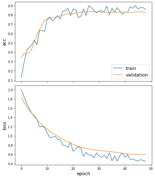
Plot the training history:
[18]:
sg.utils.plot_history(history)
Reload the saved weights of the best model found during the training (according to validation accuracy)
[19]:
model.load_weights("logs/best_model.h5")
Evaluate the best model on the test set
[20]:
test_gen = generator.flow(test_subjects.index, test_targets)
[21]:
test_metrics = model.evaluate(test_gen)
print("\nTest Set Metrics:")
for name, val in zip(model.metrics_names, test_metrics):
    print("\t{}: {:0.4f}".format(name, val))
Test Set Metrics:
        loss: 0.7227
        acc: 0.8109
Making predictions with the model
Now let’s get the predictions for all nodes:
[22]:
all_nodes = node_subjects.index
all_gen = generator.flow(all_nodes)
all_predictions = model.predict(all_gen)
These predictions will be the output of the softmax layer, so to get final categories we’ll use the inverse_transform method of our target attribute specification to turn these values back to the original categories
Note that for full-batch methods the batch size is 1 and the predictions have shape \((1, N_{nodes}, N_{classes})\) so we we remove the batch dimension to obtain predictions of shape \((N_{nodes}, N_{classes})\).
[23]:
node_predictions = target_encoding.inverse_transform(all_predictions.squeeze())
Let’s have a look at a few predictions after training the model:
[24]:
df = pd.DataFrame({"Predicted": node_predictions, "True": node_subjects})
df.head(20)
[24]:
| Predicted | True | |
|---|---|---|
| 31336 | Neural_Networks | Neural_Networks |
| 1061127 | Rule_Learning | Rule_Learning |
| 1106406 | Reinforcement_Learning | Reinforcement_Learning |
| 13195 | Reinforcement_Learning | Reinforcement_Learning |
| 37879 | Probabilistic_Methods | Probabilistic_Methods |
| 1126012 | Probabilistic_Methods | Probabilistic_Methods |
| 1107140 | Reinforcement_Learning | Theory |
| 1102850 | Neural_Networks | Neural_Networks |
| 31349 | Neural_Networks | Neural_Networks |
| 1106418 | Theory | Theory |
| 1123188 | Neural_Networks | Neural_Networks |
| 1128990 | Neural_Networks | Genetic_Algorithms |
| 109323 | Neural_Networks | Probabilistic_Methods |
| 217139 | Reinforcement_Learning | Case_Based |
| 31353 | Neural_Networks | Neural_Networks |
| 32083 | Neural_Networks | Neural_Networks |
| 1126029 | Reinforcement_Learning | Reinforcement_Learning |
| 1118017 | Neural_Networks | Neural_Networks |
| 49482 | Neural_Networks | Neural_Networks |
| 753265 | Neural_Networks | Neural_Networks |
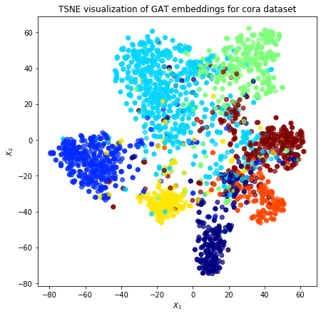
Node embeddings
Evaluate node embeddings as activations of the output of the 1st GraphAttention layer in GAT layer stack (the one before the top classification layer predicting paper subjects), and visualise them, coloring nodes by their true subject label. We expect to see nice clusters of papers in the node embedding space, with papers of the same subject belonging to the same cluster.
Let’s create a new model with the same inputs as we used previously x_inp but now the output is the embeddings rather than the predicted class. We find the embedding layer by taking the first graph attention layer in the stack of Keras layers. Additionally note that the weights trained previously are kept in the new model.
[25]:
emb_layer = next(l for l in model.layers if l.name.startswith("graph_attention"))
print(
    "Embedding layer: {}, output shape {}".format(emb_layer.name, emb_layer.output_shape)
)
Embedding layer: graph_attention_sparse, output shape (1, 2708, 64)
[26]:
embedding_model = Model(inputs=x_inp, outputs=emb_layer.output)
The embeddings can now be calculated using the predict function. Note that the embeddings returned are 64 dimensional features (8 dimensions for each of the 8 attention heads) for all nodes.
[27]:
emb = embedding_model.predict(all_gen)
emb.shape
[27]:
(1, 2708, 64)
Project the embeddings to 2d using either TSNE or PCA transform, and visualise, coloring nodes by their true subject label
[28]:
from sklearn.decomposition import PCA
from sklearn.manifold import TSNE
import pandas as pd
import numpy as np
Note that the embeddings from the GAT model have a batch dimension of 1 so we squeeze this to get a matrix of \(N_{nodes} \times N_{emb}\).
[29]:
X = emb.squeeze()
y = np.argmax(target_encoding.transform(node_subjects), axis=1)
[30]:
if X.shape[1] > 2:
    transform = TSNE  # PCA

    trans = transform(n_components=2)
    emb_transformed = pd.DataFrame(trans.fit_transform(X), index=list(G.nodes()))
    emb_transformed["label"] = y
else:
    emb_transformed = pd.DataFrame(X, index=list(G.nodes()))
    emb_transformed = emb_transformed.rename(columns={"0": 0, "1": 1})
    emb_transformed["label"] = y
[31]:
alpha = 0.7

fig, ax = plt.subplots(figsize=(7, 7))
ax.scatter(
    emb_transformed[0],
    emb_transformed[1],
    c=emb_transformed["label"].astype("category"),
    cmap="jet",
    alpha=alpha,
)
ax.set(aspect="equal", xlabel="$X_1$", ylabel="$X_2$")
plt.title(
    "{} visualization of GAT embeddings for cora dataset".format(transform.__name__)
)
plt.show()
Execute this notebook:
![]()
![]() Download locally
Download locally
