Heterogeneous GraphSAGE (HinSAGE)
This document outlines the viability and potential methodology to generalise the GraphSAGE algorithm [1] for heterogeneous graphs i.e. graphs containing many different node and edge types.
Feature updates for homogeneous graphs
The feature update rule for homogeneous graphs is, for mean aggregator:
Aggregation of features from the neighbours of node \(v\):
\({h^{k}}_{N(v)} = \frac{1}{|N(v)|}D_{p}\lbrack{h_{u}}^{k - 1}\rbrack\)
Forward pass through layer \(k\):
If
concat=True:\({h_{v}}^{k} = \sigma\left( concat\lbrack{W^{k}}_{\text{self}}D_{p}\lbrack{h_{v}}^{k - 1}\rbrack,\ {W^{k}}_{\text{neigh}}{{h}^{k}}_{N(v)}\rbrack + b^{k} \right)\)
If
concat=False:\({h_{v}}^{k} = \sigma\left( {W^{k}}_{\text{self}}D_{p}\lbrack{h_{v}}^{k - 1}\rbrack + \ {W^{k}}_{\text{neigh}}{h^{k}}_{N(v)} + b^{k} \right)\)
Where:
\({h_{v}}^{k}\) is the output for node \(v\) at layer \(k\)
\({W^{k}}_{\text{self}}\) and \({W^{k}}_{\text{neigh}}\) (both of size \(\frac{d_{k}}{2} \times d_{k - 1}\) if
concat=True, or of size \(d_{k} \times d_{k - 1}\) ifconcat=False) are trainable parameters (shared for all nodes \(v\)),\(b^{k}\) is an optional bias,
\(d_{k}\) is node feature dimensionality at layer \(k\),
\(\sigma\) is the nonlinear activation,
\(N(v)\) is the neighbourhood of node \(v\)
\(D_{p}\lbrack \cdot \rbrack\)is a random dropout with probability \(p\) applied to its argument vector.
The number of trainable parameters in layer \(k\) for the mean aggregator is
\(d_{k}d_{k - 1} + d_{k}\) if
concat=True, or\({2d}_{k}d_{k - 1} + d_{k}\) if
concat=False.
For the GCN aggregator, the feature update rule is:
- Aggregation of features from the neighbours of node \(v\):
\({h^{k}}_{N(v)} = \frac{1}{|N(v)| + 1}\left({h_{v}}^{k - 1} + \sum_{u \in N(v)}{h_{u}}^{k - 1}\right)\)
Forward pass through layer k:
\({h_{v}}^{k} = \sigma\left( W^{k} \cdot {h^{k}}_{N(v)} + b^{k} \right)\),
where \(W^{k}\) (size \(d_{k} \times d_{k - 1}\)) is a trainable weight matrix, shared between all nodes \(v\) and other notation is as for the mean aggregator.
The number of trainable parameters in layer \(k\) for the GCN
aggregator is \(d_{k}d_{k - 1} + d_{k}\), i.e., this model has the
same expressive power as the model with the mean aggregator and
concat=True, or about half the expressive power of the model with the
mean aggregator with concat=False.
Defining additional weight matrices to account for heterogeneity
To support heterogeneity of nodes and edges we propose to extend the GraphSAGE model by having separate neighbourhood weight matrices (Wneigh’s) for every unique ordered tuple of (N1, E, N2) where N1, N2 are node types, and E is an edge type. In addition the heterogeneous model will have separate self-feature matrices \(W_{\text{self}}\) for every node type (this is equivalent to having a unique self-edge type for every node type).
Note that if we enforce that every edge is only associated with a single type for the starting and ending nodes (i.e. N1 and N2 are known if E is specified) this is equivalent to having separate neighbourhood weight matrices (\(W_{\text{neigh}}\)’s) for every edge type E. However, for two node types (N1 and N2) we can have multiple edge types.
For example, to enforce that if you need a single edge of type nextTo that can either be:
Person - nextTo -> Person
Person - nextTo -> Dog
Dog - nextTo -> Person
Dog - nextTo -> Dog
you should actually define 4 different edge types such that:
Person - nextToPP -> Person
Person - nextToPD -> Dog
Dog - nextToDP -> Person
Dog - nextToDD -> Dog
Feature updates for heterogeneous graphs (HINs)
The resulting feature update rules on heterogeneous graphs, for mean and GCN aggregators, are shown below (compare with the feature update rules for homogeneous graphs above).
HinSAGE with mean aggregator
Aggregation (mean) of features from the neighbours of node \(v\) via edges of type \(r\):
\({h^{k}}_{N_{r}(v)} = \frac{1}{|N_{r}(v)|}\sum_{u \in N_r(v)}D_{p}\lbrack{h_{u}}^{k - 1}\rbrack\)
Forward pass through layer k:
If concat=Partial:
\({h_{v}}^{k} = \sigma\left( \text{concat}\lbrack{W^{k}}_{t_{v}, \text{self}}D_{p}\lbrack{h_{v}}^{k - 1}\rbrack, {W^{k}}_{r, \text{neigh}} {h^{k}}_{N_{r}(v)}\rbrack + b^{k} \right)\)
If concat=Full:
\({h_{v}}^{k} = \sigma\left( \text{concat}\lbrack{W^{k}}_{t_{v},\text{self}}D_{p}\lbrack{h_{v}}^{k - 1}\rbrack, {W^{k}}_{1,\text{neigh}} {h^{k}}_{N_{1}(v)},\ldots, {W^{k}}_{R_{e},\text{neigh}}{h^{k}}_{N_{R_{e}}(v)}\rbrack + b^{k} \right)\)
If concat=False:
\({h_{v}}^{k} = \sigma\left( {W^{k}}_{t_{v},\text{self}}D_{p}\lbrack{h_{v}}^{k - 1}\rbrack + {W^{k}}_{r,\text{neigh}}{h^{k}}_{N_{r}(v)} + b^{k} \right)\)
Where:
\({W^{k}}_{t_{v},\text{self}}\) is the weight matrix for self-edges for node type \(t_{v}\)and is of shape
\((\frac{{d_{k}}}{2}) \times d_{k - 1}\) if
concat=Partialor\(d_{k} \times d_{k - 1}\) if
concat=False, or\(\frac{d_{k}}{R_{e} + 1} \times d_{k - 1}\)if
concat=Full.\({W^{k}}_{r,\text{neigh}}\) is the weight matrix for edges of type \(r\) and is of shape
\(\frac{d_{k}}{2} \times d_{k - 1}(r)\) if
concat=Partialor\(\frac{d_{k}}{2} \times d_{k - 1}(r)\) if
concat=False, or\(\frac{d_{k}}{R_{e} + 1} \times d_{k - 1}(r)\) if
concat=Full.\(r\) denotes the edge type from node \(v\) to node \(u\) (\(r\) is defined as unique tuple \((t_{v},t_{e},t_{u})\)), where \(t_{v}\) denotes type of node \(v\), and \(t_{e}\) denotes the relation type.
\(N_{r}(v)\) is a neighbourhood of node \(v\) via edge type \(r\).
\(d_{k - 1}(r) = dim({h^{k}}_{N_{r}(v)})\) is the dimensionality of (\(k - 1\))-th layer’s features of node \(v\)’s neighbours via edge type \(r\).
The number of trainable parameters per layer \(k\) for this model is
If
concat=Partial:\(T_{v}(\frac{d_{k}}{2}) d_{k - 1} + R_{e} (\frac{d_{k}}{2})d_{k - 1} + d_{k} = \frac{T_{v} + R_{e}}{2} d_{k}d_{k - 1} + d_{k}\)
If
concat=False:\(T_{v}d_{k} d_{k - 1} + R_{e} d_{k} d_{k - 1} + d_{k} = (T_{v} + R_{e}) d_{k}d_{k - 1} + d_{k}\)
If
concat=Full\(\frac{T_{v}d_{k}}{R_{e} + 1} d_{k - 1} + R_{e} \frac{d_{k}}{R_{e} + 1}d_{k - 1} + d_{k} = d_{k}d_{k - 1}\frac{T_{v} + R_{e}}{R_{e} + 1} + d_{k}\).
assuming that the dimensionalities of all destination node features for all edge types \(r\) are all equal, i.e. \(d_{k - 1}(r) = d_{k - 1} \forall r\), the number of all node types in the graph is \(T_{v}\), and the number of all edge types is \(R_{e}\).
HinSAGE with GCN aggregator
For GCN aggregator, the feature update rule is:
Aggregation of features from the neighbours of node \(v\), and node \(v\) itself:
\({h^{k}}_{N_{r}(v)} = \frac{1}{|N_{r}(v)| + 1}\left( {h_{v}}^{k - 1} + \sum_{u \in N_r(v)}{h_{u}}^{k - 1} \right)\)
Forward pass through layer k:
\({h_{v}}^{k} = \sigma\left( \frac{1}{R_{e}}{W_{r}}^{k} \cdot {h^{k}}_{N_{r}(v)} + {b^{k}}_{} \right)\)
where \({W_{r}}^{k}\) are trainable weight matrices of size \(d_{k} \times d_{k - 1}\), one per edge type \(r\).
Note that in this model the dimensions of \({h_{u}}^{k - 1}\)for \(u \in N_{r}(v)\) for different edge types \(r\) must be the same as the dimensionality of \({h_{v}}^{k - 1}\). This can be assumed to be true after the first layer as the bias vector \(b^{k}\) in the update formula does not differ by node type.
However, if the dimensions of \({h_{u}}^{k - 1}\)for \(u \in N_{r}(v)\) differs from the size of \({h_{v}}^{k - 1}\) another weight matrix of size \(d_{k} \times d_{k - 1}(v)\) is required in front of the \({h_{v}}^{k - 1}\) term. This would be similar to the \({W^{k}}_{\text{self}}\)weight matrix of the mean aggregator.
The number of trainable parameters per layer \(k\) for this model is:
\(R_{e}d_{k}d_{k - 1} + d_{k}\)
i.e., the model with GCN aggregator is less expressive (and hence less prone to overfitting in case of small datasets) than the model with mean aggregator.
Supervised Node Attribute Inference
Although HinSAGE allows you to aggregate information from different node types, the “target” nodes for supervised attribute inference must still be of a particular node type. However, this is unlikely to be an issue since an attribute you want to infer should really only belong to a particular type of node in most cases.
Data Preparation
The input batch is best described with a diagram of an example. Given a graph schema where:
GREEN nodes have other GREEN neighbours and ORANGE neighbours
ORANGE nodes only have GREEN neighbours
and you want to infer attributes on nodes of type GREEN, you can expect a heterogeneous input batch like below:
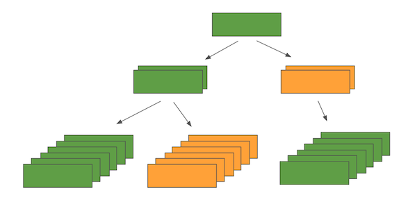
The diagram corresponds to sampling 2 neighbours at the first “hop”, and 3 neighbours at the second “hop”. From this you can imagine what the input batch should look like with arbitrary numbers of hops and number of neighbour samples at each hop. Since Keras layers only accept a list of tensors (rather than a tree) as an input, the HinSAGE layer requires an additional parameter to describe how the input list of tensors should be interpreted as a tree structure.
Additional Layers & Loss Calculation
Depending on the exact type of attribute inference you want to perform, the final classifier layer of the model may vary - e.g. binary classification, multiclass classification, regression, etc., with the corresponding loss function to be optimised. You can simply treat the output from the final layer of GraphSAGE/HinSAGE as node embeddings, and add Keras layers on top to perform the downstream task (e.g., node classification). The resulting model can then be trained end-to-end, learning the parameters of all layers at once (i.e., both the embedding layers and the final classifier/regression layer on top) via optimising the downstream task’s loss function on the training set. In this case the embeddings generated from this approach will be tailored to solve the particular downstream task they were trained for, rather than being general node embeddings (as in unsupervised GraphSAGE/HinSAGE, described below).
Unsupervised Node Feature Learning
The unsupervised representation learning with GraphSAGE/HinSAGE aims to learn general purpose node embeddings that use the graph structure as well as, optionally, the input node features. The unsupervised learning problem has connections to a link prediction problem: this makes intuitive sense since without labels the only information we have about the graph are the links. However, there are some notable differences: when training on random walks the algorithm uses pairs that are k-hop neighbours instead of actual edges, and a loss based on affinity scores is used rather than a more general edge-feature classifier.
The following formulation does not aim to be a complete solution for heterogeneous graphs, and is one way that the heterogeneity can be used to produce embeddings for a particular node type. In other words, the use-case this formulation is useful for is when you want to produce embeddings for a particular node type, but use neighbourhood information from neighbouring nodes of various types, giving the model enough expressivity to aggregate neighbours of different types more intelligently.
It is up for discussion whether it even makes sense to represent nodes of different types in one vector space. The main assumption behind this formulation of unsupervised representation learning is that neighbouring nodes have similar embeddings, and by intuition I would argue that this assumption doesn’t transfer well to a heterogeneous setting. For now, one approach to obtain embeddings for all nodes in a heterogeneous graph would be to run this model separately for each node type, but it remains to be seen whether these “separate” embeddings will be useful when applied “together” in other upstream tasks.
Data Preparation
To obtain positive pairs to train on, one of the following methods can be used:
Method 1: Use random walk target-context pairs
For each node run N random walks of length L to obtain target-context pairs. The original authors used N = 50, L = 5. It makes sense to use larger N and lower L since each context pair will be assumed as true examples of “similar nodes”.
Method 2: Use existing links
No random walks required.
Method 3 Use meta-path based random walks
For each node calculate meta-path walks of length L for M meta-path specifications, see [5].
Method 4 Use a node and its sampled k-hop neighbours
For \(k \in \{ k_{1},\ k_{2},\ k_{3},\ldots\}\)
No random walks required.
Using one of these methods, batch preparation is the same for each training loop:
src- source nodes of batch “true links/context-pairs”, and its sampled neighboursdst- destination nodes of batch “true links/context-pairs”, and its sampled neighboursdst_neg- destination nodes of batch “negative examples”, and its sampled neighbours.
Note that the dst_neg nodes are only required for the negative sampling
loss below. The skip-gram loss only requires positive pairs (src, dst).
With negative samples, compared to node attribute inference, this input
would include at least 3 times the number of nodes since every training
loop requires examples of true and false “links”. The multiplier can be
greater than 3 as there can be more than one negative pair sampled per
positive pair. In the heterogeneous case, this is likely going to blow
up, since every node might be sampling multiple different types of
neighbours - e.g. if every node had 2 types of neighbours to sample
from, then it would be \(2^{N}\) times the number of input nodes on
top of all that where N = number of neighbour hops…
Also note that src, dst, and dst_neg nodes all need to be of the same
node type, or must need to be treated as the same node type with the
same feature vector space. This is critical since the loss function
relies on the assumption that neighbouring nodes are “similar”.
Additional Layers & Loss Calculation
There are a few different loss functions implemented by the original authors, but they all use affinity scores to calculate loss. The affinity score between two given nodes is given by:
\(A(z_{u},z_{v}) = {z_{u}}^{T}z_{v}\)
This is the cosine similarity between the two embeddings \(z_{u}\) and \(z_{v}\), which simply reflects how similar they are. The learning task is typically maximizing the affinity between nodes from true context-pairs (or links), and minimizing the affinity between those from negative pairs, either implicitly in the case of the skip-gram loss or explicitly for the negative sampling loss.
Loss 1: Skip-gram loss
\(J = ({z_{u}}^{T}z_{v} - \log(e^{{z_{u}}^{T}z_{w}}))\)
This is the log-likelihood of the co-occurrence of positive pairs. This is known to be computationally intractable as the inner sum must be computed over all nodes and is therefore often approximated using hierarchical softmax [4].
Loss 2: Negative sampling loss
The default loss function given by the original author’s implementation. This is a binary cross-entropy loss where positive target-context pairs have a label of 1, and negative sample pairs have a label of zero, and take the sum, with an optional weight on the component from negative examples. This simplifies to the below expression:
\(J = - \log(\sigma({z_{u}}^{T}z_{v})) - \log(\sigma( - {z_{u}}^{T}z_{v_{n}}))\)
where
\(\sigma(x) = \frac{1}{1 + e^{- x}}\) is the sigmoid function
\((u,v)\) and \((u,v_{n})\) are positive and negative pairs respectively.
Heterogeneous loss functions
In the case of heterogeneous graph, the loss functions for unsupervised learning can be formulated to consider different node and edge types.
Supervised Link Prediction
As mentioned in the previous section, link prediction is similar to how unsupervised GraphSAGE/HinSAGE is formulated. Similar to the way unsupervised learning was restricted to learning embeddings for a particular node type in a heterogeneous setting, the link prediction algorithm is also limited to learning links of a particular type. However, this is likely to be less of an issue since you could argue that most link prediction problems are interested in predicting a particular link type anyway. Also note that there’s no constraint on the source and destination node types - i.e. you could predict links that have different source and destination node types, as long as you are predicting that particular link type.
Data Preparation
Identical to method 2 of the unsupervised learning data preparation, except for the fact that you are taking positive and negative examples of a particular link type which has consistent source and destination node types.
Additional Layers & Loss Calculation
If we treat the output from the GraphSAGE layers as node embeddings for the source and destination nodes, then we need to combine these embeddings with a binary operator to obtain embeddings that correspond to links. For directed edges, we could expect concatenation to produce reasonable embeddings. Each of these edges can then be fed through a simple classifier, and calculate cross entropy against a vector of ones for true edges and zeros for negative examples.
\(J = ( - \log(\sigma(concat(z_{u}, z_{v})))) + ( - \log(\sigma( - concat(z_{u},z_{v_{n}}))))\)
References
[1] W. L. Hamilton, R. Ying, and J. Leskovec, “Inductive Representation Learning on Large Graphs,” arXiv.org. 08-Jun-2017.
[2] J. Chen, T. Ma, and C. Xiao, “FastGCN: Fast Learning with Graph Convolutional Networks via Importance Sampling,” arXiv.org, vol. cs.LG. 31-Jan-2018.
[3] J. Chen, J. Zhu, and Le Song, “Stochastic Training of Graph Convolutional Networks with Variance Reduction,” arXiv.org, vol. stat.ML. 29-Oct-2017.
[4] B. Perozzi, R. Al-Rfou, and S. Skiena, “DeepWalk: Online Learning of Social Representations,” presented at the ACM SIGKDD international conference on Knowledge discovery and data mining, New York, New York, USA, 2014, pp. 701–710.
[5] J. Shang, M. Qu, J. Liu, L. M. Kaplan, J. Han, and J. Peng, “Meta-Path Guided Embedding for Similarity Search in Large-Scale Heterogeneous Information Networks,” arXiv.org, vol. cs.SI. 31-Oct-2016.
