Execute this notebook:
![]()
![]() Download locally
Download locally
Node classification with Node2Vec using Stellargraph components
This example demonstrates how to perform node classification with Node2Vec using the Stellargraph components. This uses a Keras implementation of Node2Vec available in stellargraph instead of the reference implementation provided by gensim.
References
[1] Node2Vec: Scalable Feature Learning for Networks. A. Grover, J. Leskovec. ACM SIGKDD International Conference on Knowledge Discovery and Data Mining (KDD), 2016. (link)
[2] Distributed representations of words and phrases and their compositionality. T. Mikolov, I. Sutskever, K. Chen, G. S. Corrado, and J. Dean. In Advances in Neural Information Processing Systems (NIPS), pp. 3111-3119, 2013. (link)
[3] word2vec Parameter Learning Explained. X. Rong. arXiv preprint arXiv:1411.2738. 2014 Nov 11. (link)
Introduction
Following word2vec [2,3], for each (target,context) node pair \((v_i,v_j)\) collected from random walks, we learn the representation for the target node \(v_i\) by using it to predict the existence of context node \(v_j\), with the following three-layer neural network.
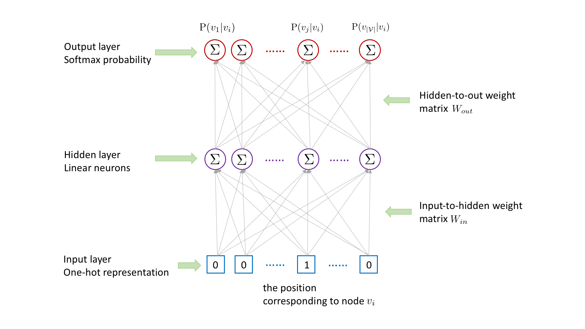
Node \(v_i\)’s representation in the hidden layer is obtained by multiplying \(v_i\)’s one-hot representation in the input layer with the input-to-hidden weight matrix \(W_{in}\), which is equivalent to look up the \(i\)th row of input-to-hidden weight matrix \(W_{in}\). The existence probability of each node conditioned on node \(v_i\) is outputted in the output layer, which is obtained by multiplying \(v_i\)’s hidden-layer representation with the hidden-to-out
weight matrix \(W_{out}\) followed by a softmax activation. To capture the target-context relation between \(v_i\) and \(v_j\), we need to maximize the probability \(\mathrm{P}(v_j|v_i)\). However, computing \(\mathrm{P}(v_j|v_i)\) is time consuming, which involves the matrix multiplication between \(v_i\)’s hidden-layer representation and the hidden-to-out weight matrix \(W_{out}\).
To speed up the computing, we adopt the negative sampling strategy [2,3]. For each (target, context) node pair, we sample a negative node \(v_k\), which is not \(v_i\)’s context. To obtain the output, instead of multiplying \(v_i\)’s hidden-layer representation with the hidden-to-out weight matrix \(W_{out}\) followed by a softmax activation, we only calculate the dot product between \(v_i\)’s hidden-layer representation and the \(j\)th column as well as the
\(k\)th column of the hidden-to-output weight matrix \(W_{out}\) followed by a sigmoid activation respectively. According to [3], the original objective to maximize \(\mathrm{P}(v_j|v_i)\) can be approximated by minimizing the cross entropy between \(v_j\) and \(v_k\)’s outputs and their ground-truth labels (1 for \(v_j\) and 0 for \(v_k\)).
Following [2,3], we denote the rows of the input-to-hidden weight matrix \(W_{in}\) as input_embeddings and the columns of the hidden-to-out weight matrix \(W_{out}\) as output_embeddings. To build the Node2Vec model, we need look up input_embeddings for target nodes and output_embeddings for context nodes and calculate their inner product together with a sigmoid activation.
[3]:
import matplotlib.pyplot as plt

from sklearn.manifold import TSNE
from sklearn.model_selection import train_test_split
from sklearn.linear_model import LogisticRegressionCV
from sklearn.metrics import accuracy_score

import os
import networkx as nx
import numpy as np
import pandas as pd
from tensorflow import keras

from stellargraph import StellarGraph
from stellargraph.data import BiasedRandomWalk
from stellargraph.data import UnsupervisedSampler
from stellargraph.data import BiasedRandomWalk
from stellargraph.mapper import Node2VecLinkGenerator, Node2VecNodeGenerator
from stellargraph.layer import Node2Vec, link_classification

from stellargraph import datasets
from IPython.display import display, HTML

%matplotlib inline
Dataset
For clarity, we use only the largest connected component, ignoring isolated nodes and subgraphs; having these in the data does not prevent the algorithm from running and producing valid results.
[4]:
dataset = datasets.Cora()
display(HTML(dataset.description))
G, subjects = dataset.load(largest_connected_component_only=True)
[5]:
print(G.info())
StellarGraph: Undirected multigraph
 Nodes: 2485, Edges: 5209

 Node types:
  paper: [2485]
    Features: float32 vector, length 1433
    Edge types: paper-cites->paper

 Edge types:
    paper-cites->paper: [5209]
        Weights: all 1 (default)
        Features: none
The Node2Vec algorithm
The Node2Vec algorithm introduced in [1] is a 2-step representation learning algorithm. The two steps are:
Use random walks to generate sentences from a graph. A sentence is a list of node ids. The set of all sentences makes a corpus.
The corpus is then used to learn an embedding vector for each node in the graph. Each node id is considered a unique word/token in a dictionary that has size equal to the number of nodes in the graph. The Word2Vec algorithm [2] is used for calculating the embedding vectors.
In this implementation, we train the Node2Vec algorithm in the following two steps:
Generate a set of (
target,context) node pairs through starting the biased random walk with a fixed length at per node. The starting nodes are taken as the target nodes and the following nodes in biased random walks are taken as context nodes. For each (target,context) node pair, we generate 1 negative node pair.Train the Node2Vec algorithm through minimizing cross-entropy loss for
target-contextpair prediction, with the predictive value obtained by performing the dot product of the ‘input embedding’ of the target node and the ‘output embedding’ of the context node, followed by a sigmoid activation.
Specify the optional parameter values: the number of walks to take per node, the length of each walk. Here, to guarantee the running efficiency, we respectively set walk_number and walk_length to 100 and 5. Larger values can be set to them to achieve better performance.
[6]:
walk_number = 100
walk_length = 5
Create the biased random walker to perform context node sampling, with the specified parameters.
[7]:
walker = BiasedRandomWalk(
    G,
    n=walk_number,
    length=walk_length,
    p=0.5,  # defines probability, 1/p, of returning to source node
    q=2.0,  # defines probability, 1/q, for moving to a node away from the source node
)
Create the UnsupervisedSampler instance with the biased random walker.
[8]:
unsupervised_samples = UnsupervisedSampler(G, nodes=list(G.nodes()), walker=walker)
Set the batch size and the number of epochs.
[9]:
batch_size = 50
epochs = 2
Define an attri2vec training generator, which generates a batch of (index of target node, index of context node, label of node pair) pairs per iteration.
[10]:
generator = Node2VecLinkGenerator(G, batch_size)
Build the Node2Vec model, with the dimension of learned node representations set to 128.
[11]:
emb_size = 128
node2vec = Node2Vec(emb_size, generator=generator)
[12]:
x_inp, x_out = node2vec.in_out_tensors()
Use the link_classification function to generate the prediction, with the ‘dot’ edge embedding generation method and the ‘sigmoid’ activation, which actually performs the dot product of the ‘input embedding’ of the target node and the ‘output embedding’ of the context node followed by a sigmoid activation.
[13]:
prediction = link_classification(
    output_dim=1, output_act="sigmoid", edge_embedding_method="dot"
)(x_out)
link_classification: using 'dot' method to combine node embeddings into edge embeddings
Stack the Node2Vec encoder and prediction layer into a Keras model. Our generator will produce batches of positive and negative context pairs as inputs to the model. Minimizing the binary crossentropy between the outputs and the provided ground truth is much like a regular binary classification task.
[14]:
model = keras.Model(inputs=x_inp, outputs=prediction)

model.compile(
    optimizer=keras.optimizers.Adam(lr=1e-3),
    loss=keras.losses.binary_crossentropy,
    metrics=[keras.metrics.binary_accuracy],
)
Train the model.
[15]:
history = model.fit(
    generator.flow(unsupervised_samples),
    epochs=epochs,
    verbose=1,
    use_multiprocessing=False,
    workers=4,
    shuffle=True,
)
Train for 39760 steps
Epoch 1/2
39760/39760 [==============================] - 156s 4ms/step - loss: 0.2969 - binary_accuracy: 0.8529
Epoch 2/2
39760/39760 [==============================] - 240s 6ms/step - loss: 0.1087 - binary_accuracy: 0.9643
Visualise Node Embeddings
Build the node based model for predicting node representations from node ids and the learned parameters. Below a Keras model is constructed, with x_inp[0] as input and x_out[0] as output. Note that this model’s weights are the same as those of the corresponding node encoder in the previously trained node pair classifier.
[16]:
x_inp_src = x_inp[0]
x_out_src = x_out[0]
embedding_model = keras.Model(inputs=x_inp_src, outputs=x_out_src)
Get the node embeddings from node ids.
[17]:
node_gen = Node2VecNodeGenerator(G, batch_size).flow(subjects.index)
node_embeddings = embedding_model.predict(node_gen, workers=4, verbose=1)
50/50 [==============================] - 0s 1ms/step
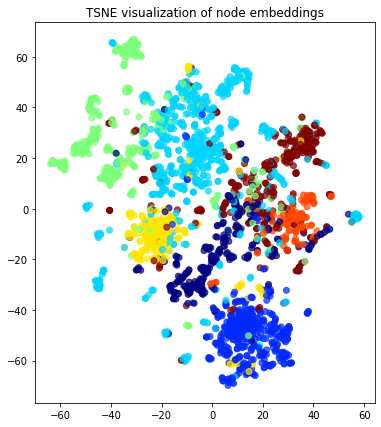
Transform the embeddings to 2d space for visualisation.
[18]:
transform = TSNE  # PCA

trans = transform(n_components=2)
node_embeddings_2d = trans.fit_transform(node_embeddings)
[19]:
# draw the embedding points, coloring them by the target label (paper subject)
alpha = 0.7
label_map = {l: i for i, l in enumerate(np.unique(subjects))}
node_colours = [label_map[target] for target in subjects]

plt.figure(figsize=(7, 7))
plt.axes().set(aspect="equal")
plt.scatter(
    node_embeddings_2d[:, 0],
    node_embeddings_2d[:, 1],
    c=node_colours,
    cmap="jet",
    alpha=alpha,
)
plt.title("{} visualization of node embeddings".format(transform.__name__))
plt.show()
Node Classification
In this task, we will use the Node2Vec node embeddings to train a classifier to predict the subject of a paper in Cora.
[20]:
# X will hold the 128-dimensional input features
X = node_embeddings
# y holds the corresponding target values
y = np.array(subjects)
Data Splitting
We split the data into train and test sets.
We use 10% of the data for training and the remaining 90% for testing as a hold-out test set.
[21]:
X_train, X_test, y_train, y_test = train_test_split(X, y, train_size=0.1, test_size=None)
print(
    "Array shapes:\n X_train = {}\n y_train = {}\n X_test = {}\n y_test = {}".format(
        X_train.shape, y_train.shape, X_test.shape, y_test.shape
    )
)
Array shapes:
 X_train = (248, 128)
 y_train = (248,)
 X_test = (2237, 128)
 y_test = (2237,)
Classifier Training
We train a Logistic Regression classifier on the training data.
[22]:
clf = LogisticRegressionCV(
    Cs=10, cv=10, scoring="accuracy", verbose=False, multi_class="ovr", max_iter=300
)
clf.fit(X_train, y_train)
[22]:
LogisticRegressionCV(Cs=10, class_weight=None, cv=10, dual=False,
                     fit_intercept=True, intercept_scaling=1.0, l1_ratios=None,
                     max_iter=300, multi_class='ovr', n_jobs=None, penalty='l2',
                     random_state=None, refit=True, scoring='accuracy',
                     solver='lbfgs', tol=0.0001, verbose=False)
Predict the hold-out test set.
[23]:
y_pred = clf.predict(X_test)
Calculate the accuracy of the classifier on the test set.
[24]:
accuracy_score(y_test, y_pred)
[24]:
0.7358068842199375
Execute this notebook:
![]()
![]() Download locally
Download locally
