Execute this notebook: Download locally

Supervised graph classification with GCN

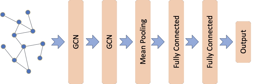
This notebook demonstrates how to train a graph classification model in a supervised setting using graph convolutional layers followed by a mean pooling layer as well as any number of fully connected layers.

The graph convolutional classification model architecture is based on the one proposed in [1] (see Figure 5 in [1]) using the graph convolutional layers from [2]. This demo differs from [1] in the dataset, MUTAG, used here; MUTAG is a collection of static graphs representing chemical compounds with each graph associated with a binary label. Furthermore, none of the graph convolutional layers in our model utilise an attention head as proposed in [1].

Evaluation data for graph kernel-based approaches shown in the very last cell in this notebook are taken from [3].

References

[1] Fake News Detection on Social Media using Geometric Deep Learning, F. Monti, F. Frasca, D. Eynard, D. Mannion, and M. M. Bronstein, ICLR 2019. (link)

[2] Semi-supervised Classification with Graph Convolutional Networks, T. N. Kipf and M. Welling, ICLR 2017. (link)

[3] An End-to-End Deep Learning Architecture for Graph Classification, M. Zhang, Z. Cui, M. Neumann, Y. Chen, AAAI-18. (link)

import pandas as pd
import numpy as np

import stellargraph as sg
from stellargraph.mapper import PaddedGraphGenerator
from stellargraph.layer import GCNSupervisedGraphClassification
from stellargraph import StellarGraph

from stellargraph import datasets

from sklearn import model_selection
from IPython.display import display, HTML

from tensorflow.keras import Model
from tensorflow.keras.optimizers import Adam
from tensorflow.keras.layers import Dense
from tensorflow.keras.losses import binary_crossentropy
from tensorflow.keras.callbacks import EarlyStopping
import tensorflow as tf
import matplotlib.pyplot as plt

Import the data

(See the “Loading from Pandas” demo for details on how data can be loaded.)

dataset = datasets.MUTAG()
display(HTML(dataset.description))
graphs, graph_labels = dataset.load()

Each graph represents a chemical compound and graph labels represent 'their mutagenic effect on a specific gram negative bacterium.'The dataset includes 188 graphs with 18 nodes and 20 edges on average for each graph. Graph nodes have 7 labels and each graph is labelled as belonging to 1 of 2 classes.

The graphs value is a list of many StellarGraph instances, each of which has a few node features:

print(graphs[0].info())

StellarGraph: Undirected multigraph
 Nodes: 17, Edges: 38

 Node types:
  default: [17]
    Features: float32 vector, length 7
    Edge types: default-default->default

 Edge types:
    default-default->default: [38]
        Weights: all 1 (default)
        Features: none

print(graphs[1].info())

StellarGraph: Undirected multigraph
 Nodes: 13, Edges: 28

 Node types:
  default: [13]
    Features: float32 vector, length 7
    Edge types: default-default->default

 Edge types:
    default-default->default: [28]
        Weights: all 1 (default)
        Features: none

Summary statistics of the sizes of the graphs:

summary = pd.DataFrame(
    [(g.number_of_nodes(), g.number_of_edges()) for g in graphs],
    columns=["nodes", "edges"],
)
summary.describe().round(1)

	nodes	edges
count	188.0	188.0
mean	17.9	39.6
std	4.6	11.4
min	10.0	20.0
25%	14.0	28.0
50%	17.5	38.0
75%	22.0	50.0
max	28.0	66.0

The labels are 1 or -1:

graph_labels.value_counts().to_frame()

	label
1	125
-1	63

graph_labels = pd.get_dummies(graph_labels, drop_first=True)

Prepare graph generator

To feed data to the tf.Keras model that we will create later, we need a data generator. For supervised graph classification, we create an instance of StellarGraph’s PaddedGraphGenerator class. Note that graphs is a list of StellarGraph graph objects.

generator = PaddedGraphGenerator(graphs=graphs)

Create the Keras graph classification model

We are now ready to create a tf.Keras graph classification model using StellarGraph’s GraphClassification class together with standard tf.Keras layers, e.g., Dense.

The input is the graph represented by its adjacency and node features matrices. The first two layers are Graph Convolutional as in [2] with each layer having 64 units and relu activations. The next layer is a mean pooling layer where the learned node representation are summarized to create a graph representation. The graph representation is input to two fully connected layers with 32 and 16 units respectively and relu activations. The last layer is the output layer with a single unit and sigmoid activation.

def create_graph_classification_model(generator):
    gc_model = GCNSupervisedGraphClassification(
        layer_sizes=[64, 64],
        activations=["relu", "relu"],
        generator=generator,
        dropout=0.5,
    )
    x_inp, x_out = gc_model.in_out_tensors()
    predictions = Dense(units=32, activation="relu")(x_out)
    predictions = Dense(units=16, activation="relu")(predictions)
    predictions = Dense(units=1, activation="sigmoid")(predictions)

    # Let's create the Keras model and prepare it for training
    model = Model(inputs=x_inp, outputs=predictions)
    model.compile(optimizer=Adam(0.005), loss=binary_crossentropy, metrics=["acc"])

    return model

Train the model

We can now train the model using the model’s fit method. First, we specify some important training parameters such as the number of training epochs, number of fold for cross validation and the number of time to repeat cross validation.

epochs = 200  # maximum number of training epochs
folds = 10  # the number of folds for k-fold cross validation
n_repeats = 5  # the number of repeats for repeated k-fold cross validation

es = EarlyStopping(
    monitor="val_loss", min_delta=0, patience=25, restore_best_weights=True
)

The method train_fold is used to train a graph classification model for a single fold of the data.

def train_fold(model, train_gen, test_gen, es, epochs):
    history = model.fit(
        train_gen, epochs=epochs, validation_data=test_gen, verbose=0, callbacks=[es],
    )
    # calculate performance on the test data and return along with history
    test_metrics = model.evaluate(test_gen, verbose=0)
    test_acc = test_metrics[model.metrics_names.index("acc")]

    return history, test_acc

def get_generators(train_index, test_index, graph_labels, batch_size):
    train_gen = generator.flow(
        train_index, targets=graph_labels.iloc[train_index].values, batch_size=batch_size
    )
    test_gen = generator.flow(
        test_index, targets=graph_labels.iloc[test_index].values, batch_size=batch_size
    )

    return train_gen, test_gen

The code below puts all the above functionality together in a training loop for repeated k-fold cross-validation where the number of folds is 10, folds=10; that is we do 10-fold cross validation n_repeats times where n_repeats=5.

Note: The below code may take a long time to run depending on the value set for n_repeats. The larger the latter, the longer it takes since for each repeat we train and evaluate 10 graph classification models, one for each fold of the data. For progress updates, we recommend that you set verbose=2 in the call to the fit method is cell 10, line 3.

test_accs = []

stratified_folds = model_selection.RepeatedStratifiedKFold(
    n_splits=folds, n_repeats=n_repeats
).split(graph_labels, graph_labels)

for i, (train_index, test_index) in enumerate(stratified_folds):
    print(f"Training and evaluating on fold {i+1} out of {folds * n_repeats}...")
    train_gen, test_gen = get_generators(
        train_index, test_index, graph_labels, batch_size=30
    )

    model = create_graph_classification_model(generator)

    history, acc = train_fold(model, train_gen, test_gen, es, epochs)

    test_accs.append(acc)

Training and evaluating on fold 1 out of 50...
  ['...']
  ['...']
  ['...']
Training and evaluating on fold 2 out of 50...
  ['...']
  ['...']
  ['...']
Training and evaluating on fold 3 out of 50...
  ['...']
  ['...']
  ['...']
Training and evaluating on fold 4 out of 50...
  ['...']
  ['...']
  ['...']
Training and evaluating on fold 5 out of 50...
  ['...']
  ['...']
  ['...']
Training and evaluating on fold 6 out of 50...
  ['...']
  ['...']
  ['...']
Training and evaluating on fold 7 out of 50...
  ['...']
  ['...']
  ['...']
Training and evaluating on fold 8 out of 50...
  ['...']
  ['...']
  ['...']
Training and evaluating on fold 9 out of 50...
  ['...']
  ['...']
  ['...']
Training and evaluating on fold 10 out of 50...
  ['...']
  ['...']
  ['...']
Training and evaluating on fold 11 out of 50...
  ['...']
  ['...']
  ['...']
Training and evaluating on fold 12 out of 50...
  ['...']
  ['...']
  ['...']
Training and evaluating on fold 13 out of 50...
  ['...']
  ['...']
  ['...']
Training and evaluating on fold 14 out of 50...
  ['...']
  ['...']
  ['...']
Training and evaluating on fold 15 out of 50...
  ['...']
  ['...']
  ['...']
Training and evaluating on fold 16 out of 50...
  ['...']
  ['...']
  ['...']
Training and evaluating on fold 17 out of 50...
  ['...']
  ['...']
  ['...']
Training and evaluating on fold 18 out of 50...
  ['...']
  ['...']
  ['...']
Training and evaluating on fold 19 out of 50...
  ['...']
  ['...']
  ['...']
Training and evaluating on fold 20 out of 50...
  ['...']
  ['...']
  ['...']
Training and evaluating on fold 21 out of 50...
  ['...']
  ['...']
  ['...']
Training and evaluating on fold 22 out of 50...
  ['...']
  ['...']
  ['...']
Training and evaluating on fold 23 out of 50...
  ['...']
  ['...']
  ['...']
Training and evaluating on fold 24 out of 50...
  ['...']
  ['...']
  ['...']
Training and evaluating on fold 25 out of 50...
  ['...']
  ['...']
  ['...']
Training and evaluating on fold 26 out of 50...
  ['...']
  ['...']
  ['...']
Training and evaluating on fold 27 out of 50...
  ['...']
  ['...']
  ['...']
Training and evaluating on fold 28 out of 50...
  ['...']
  ['...']
  ['...']
Training and evaluating on fold 29 out of 50...
  ['...']
  ['...']
  ['...']
Training and evaluating on fold 30 out of 50...
  ['...']
  ['...']
  ['...']
Training and evaluating on fold 31 out of 50...
  ['...']
  ['...']
  ['...']
Training and evaluating on fold 32 out of 50...
  ['...']
  ['...']
  ['...']
Training and evaluating on fold 33 out of 50...
  ['...']
  ['...']
  ['...']
Training and evaluating on fold 34 out of 50...
  ['...']
  ['...']
  ['...']
Training and evaluating on fold 35 out of 50...
  ['...']
  ['...']
  ['...']
Training and evaluating on fold 36 out of 50...
  ['...']
  ['...']
  ['...']
Training and evaluating on fold 37 out of 50...
  ['...']
  ['...']
  ['...']
Training and evaluating on fold 38 out of 50...
  ['...']
  ['...']
  ['...']
Training and evaluating on fold 39 out of 50...
  ['...']
  ['...']
  ['...']
Training and evaluating on fold 40 out of 50...
  ['...']
  ['...']
  ['...']
Training and evaluating on fold 41 out of 50...
  ['...']
  ['...']
  ['...']
Training and evaluating on fold 42 out of 50...
  ['...']
  ['...']
  ['...']
Training and evaluating on fold 43 out of 50...
  ['...']
  ['...']
  ['...']
Training and evaluating on fold 44 out of 50...
  ['...']
  ['...']
  ['...']
Training and evaluating on fold 45 out of 50...
  ['...']
  ['...']
  ['...']
Training and evaluating on fold 46 out of 50...
  ['...']
  ['...']
  ['...']
Training and evaluating on fold 47 out of 50...
  ['...']
  ['...']
  ['...']
Training and evaluating on fold 48 out of 50...
  ['...']
  ['...']
  ['...']
Training and evaluating on fold 49 out of 50...
  ['...']
  ['...']
  ['...']
Training and evaluating on fold 50 out of 50...
  ['...']
  ['...']
  ['...']

print(
    f"Accuracy over all folds mean: {np.mean(test_accs)*100:.3}% and std: {np.std(test_accs)*100:.2}%"
)

Accuracy over all folds mean: 76.4% and std: 6.7%

Finally, we plot a histogram of the accuracy of all n_repeats x folds models trained (50 in total).

plt.figure(figsize=(8, 6))
plt.hist(test_accs)
plt.xlabel("Accuracy")
plt.ylabel("Count")

Text(0, 0.5, 'Count')

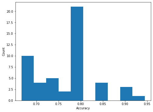
The histogram shown above indicates the difficulty of training a good model on the MUTAG dataset due to the following factors, - small amount of available data, i.e., only 188 graphs - small amount of validation data since for a single fold only 19 graphs are used for validation - the data are unbalanced since the majority class is twice as prevalent in the data

Given the above, average performance as estimated using repeated 10-fold cross validation displays high variance but overall good performance for a straightforward application of graph convolutional neural networks to supervised graph classification. The high variance is likely the result of the small dataset size.

Generally, performance is a bit lower than SOTA in recent literature. However, we have not tuned the model for the best performance possible so some improvement over the current baseline may be attainable.

When comparing to graph kernel-based approaches, our straightforward GCN with mean pooling graph classification model is competitive with the WL kernel being the exception.

For comparison, some performance numbers repeated from [3] for graph kernel-based approaches are, - Graphlet Kernel (GK): \(81.39\pm1.74\) - Random Walk Kernel (RW): \(79.17\pm2.07\) - Propagation Kernel (PK): \(76.00\pm2.69\) - Weisfeiler-Lehman Subtree Kernel (WL): \(84.11\pm1.91\)

Execute this notebook: Download locally