Execute this notebook:
![]()
![]() Download locally
Download locally
Supervised graph classification with Deep Graph CNN
This notebook demonstrates how to train a graph classification model in a supervised setting using the Deep Graph Convolutional Neural Network (DGCNN) [1] algorithm.
In supervised graph classification, we are given a collection of graphs each with an attached categorical label. For example, the PROTEINS dataset we use for this demo is a collection of graphs each representing a chemical compound and labelled as either an enzyme or not. Our goal is to train a machine learning model that uses the graph structure of the data together with any information available for the graph’s nodes, e.g., chemical properties for the compounds in PROTEINS, to predict the correct label for a previously unseen graph; a previously unseen graph is one that was not used for training and validating the model.
The DGCNN architecture was proposed in [1] (see Figure 5 in [1]) using the graph convolutional layers from [2] but with a modified propagation rule (see [1] for details). DGCNN introduces a new SortPooling layer to generate a representation (also know as embedding) for each given graph using as input the representations learned for each node via a stack of graph convolutional layers. The output of the SortPooling layer is then used as input to one-dimensional convolutional, max pooling,
and dense layers that learn graph-level features suitable for predicting graph labels.
References
[1] An End-to-End Deep Learning Architecture for Graph Classification, M. Zhang, Z. Cui, M. Neumann, Y. Chen, AAAI-18. (link)
[2] Semi-supervised Classification with Graph Convolutional Networks, T. N. Kipf and M. Welling, ICLR 2017. (link)
[3]:
import pandas as pd
import numpy as np

import stellargraph as sg
from stellargraph.mapper import PaddedGraphGenerator
from stellargraph.layer import DeepGraphCNN
from stellargraph import StellarGraph

from stellargraph import datasets

from sklearn import model_selection
from IPython.display import display, HTML

from tensorflow.keras import Model
from tensorflow.keras.optimizers import Adam
from tensorflow.keras.layers import Dense, Conv1D, MaxPool1D, Dropout, Flatten
from tensorflow.keras.losses import binary_crossentropy
import tensorflow as tf
Import the data
(See the “Loading from Pandas” demo for details on how data can be loaded.)
[4]:
dataset = datasets.PROTEINS()
display(HTML(dataset.description))
graphs, graph_labels = dataset.load()
The graphs value is a list of many StellarGraph instances, each of which has a few node features:
[5]:
print(graphs[0].info())
StellarGraph: Undirected multigraph
 Nodes: 42, Edges: 162

 Node types:
  default: [42]
    Features: float32 vector, length 4
    Edge types: default-default->default

 Edge types:
    default-default->default: [162]
        Weights: all 1 (default)
        Features: none
[6]:
print(graphs[1].info())
StellarGraph: Undirected multigraph
 Nodes: 27, Edges: 92

 Node types:
  default: [27]
    Features: float32 vector, length 4
    Edge types: default-default->default

 Edge types:
    default-default->default: [92]
        Weights: all 1 (default)
        Features: none
Summary statistics of the sizes of the graphs:
[7]:
summary = pd.DataFrame(
    [(g.number_of_nodes(), g.number_of_edges()) for g in graphs],
    columns=["nodes", "edges"],
)
summary.describe().round(1)
[7]:
| nodes | edges | |
|---|---|---|
| count | 1113.0 | 1113.0 |
| mean | 39.1 | 145.6 |
| std | 45.8 | 169.3 |
| min | 4.0 | 10.0 |
| 25% | 15.0 | 56.0 |
| 50% | 26.0 | 98.0 |
| 75% | 45.0 | 174.0 |
| max | 620.0 | 2098.0 |
The labels are 1 or 2:
[8]:
graph_labels.value_counts().to_frame()
[8]:
| label | |
|---|---|
| 1 | 663 |
| 2 | 450 |
[9]:
graph_labels = pd.get_dummies(graph_labels, drop_first=True)
Prepare graph generator
To feed data to the tf.Keras model that we will create later, we need a data generator. For supervised graph classification, we create an instance of StellarGraph’s PaddedGraphGenerator class.
[10]:
generator = PaddedGraphGenerator(graphs=graphs)
Create the Keras graph classification model
We are now ready to create a tf.Keras graph classification model using StellarGraph’s DeepGraphCNN class together with standard tf.Keras layers Conv1D, MapPool1D, Dropout, and Dense.
The model’s input is the graph represented by its adjacency and node features matrices. The first four layers are Graph Convolutional as in [2] but using the adjacency normalisation from [1], \(D^{-1}A\) where \(A\) is the adjacency matrix with self loops and \(D\) is the corresponding degree matrix. The graph convolutional layers each have 32, 32, 32, 1 units and tanh activations.
The next layer is a one dimensional convolutional layer, Conv1D, followed by a max pooling, MaxPool1D, layer. Next is a second Conv1D layer that is followed by two Dense layers the second used for binary classification. The convolutional and dense layers use relu activation except for the last dense layer that uses sigmoid for classification. As described in [1], we add a Dropout layer after the first Dense layer.
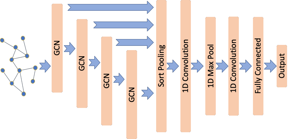
First we create the base DGCNN model that includes the graph convolutional and SortPooling layers.
[11]:
k = 35  # the number of rows for the output tensor
layer_sizes = [32, 32, 32, 1]

dgcnn_model = DeepGraphCNN(
    layer_sizes=layer_sizes,
    activations=["tanh", "tanh", "tanh", "tanh"],
    k=k,
    bias=False,
    generator=generator,
)
x_inp, x_out = dgcnn_model.in_out_tensors()
Next, we add the convolutional, max pooling, and dense layers.
[12]:
x_out = Conv1D(filters=16, kernel_size=sum(layer_sizes), strides=sum(layer_sizes))(x_out)
x_out = MaxPool1D(pool_size=2)(x_out)

x_out = Conv1D(filters=32, kernel_size=5, strides=1)(x_out)

x_out = Flatten()(x_out)

x_out = Dense(units=128, activation="relu")(x_out)
x_out = Dropout(rate=0.5)(x_out)

predictions = Dense(units=1, activation="sigmoid")(x_out)
Finally, we create the Keras model and prepare it for training by specifying the loss and optimisation algorithm.
[13]:
model = Model(inputs=x_inp, outputs=predictions)

model.compile(
    optimizer=Adam(lr=0.0001), loss=binary_crossentropy, metrics=["acc"],
)
Train the model
We can now train the model using the model’s fit method.
But first we need to split our data to training and test sets. We are going to use 90% of the data for training and the remaining 10% for testing. This 90/10 split is the equivalent of a single fold in the 10-fold cross validation scheme used in [1].
[14]:
train_graphs, test_graphs = model_selection.train_test_split(
    graph_labels, train_size=0.9, test_size=None, stratify=graph_labels,
)
Given the data split into train and test sets, we create a StellarGraph.PaddedGenerator generator object that prepares the data for training. We create data generators suitable for training at tf.keras model by calling the latter generator’s flow method specifying the train and test data.
[15]:
gen = PaddedGraphGenerator(graphs=graphs)

train_gen = gen.flow(
    list(train_graphs.index - 1),
    targets=train_graphs.values,
    batch_size=50,
    symmetric_normalization=False,
)

test_gen = gen.flow(
    list(test_graphs.index - 1),
    targets=test_graphs.values,
    batch_size=1,
    symmetric_normalization=False,
)
Note: We set the number of epochs to a large value so the call to model.fit(...) later might take a long time to complete. For faster performance set epochs to a smaller value; but if you do accuracy of the model found may be low.
[16]:
epochs = 100
We can now train the model by calling it’s fit method.
[17]:
history = model.fit(
    train_gen, epochs=epochs, verbose=1, validation_data=test_gen, shuffle=True,
)
  ['...']
  ['...']
Train for 21 steps, validate for 112 steps
Epoch 1/100
21/21 [==============================] - 3s 139ms/step - loss: 0.6640 - acc: 0.5824 - val_loss: 0.6188 - val_acc: 0.5982
Epoch 2/100
21/21 [==============================] - 2s 74ms/step - loss: 0.6526 - acc: 0.6234 - val_loss: 0.6003 - val_acc: 0.6429
Epoch 3/100
21/21 [==============================] - 2s 86ms/step - loss: 0.6468 - acc: 0.6643 - val_loss: 0.5987 - val_acc: 0.7411
Epoch 4/100
21/21 [==============================] - 2s 76ms/step - loss: 0.6361 - acc: 0.7123 - val_loss: 0.5843 - val_acc: 0.7321
Epoch 5/100
21/21 [==============================] - 2s 83ms/step - loss: 0.6301 - acc: 0.7143 - val_loss: 0.5786 - val_acc: 0.7500
Epoch 6/100
21/21 [==============================] - 2s 86ms/step - loss: 0.6061 - acc: 0.7073 - val_loss: 0.5716 - val_acc: 0.7500
Epoch 7/100
21/21 [==============================] - 2s 81ms/step - loss: 0.6129 - acc: 0.7173 - val_loss: 0.5626 - val_acc: 0.7500
Epoch 8/100
21/21 [==============================] - 2s 82ms/step - loss: 0.6274 - acc: 0.7163 - val_loss: 0.5637 - val_acc: 0.7411
Epoch 9/100
21/21 [==============================] - 2s 84ms/step - loss: 0.5985 - acc: 0.7243 - val_loss: 0.5606 - val_acc: 0.7411
Epoch 10/100
21/21 [==============================] - 2s 86ms/step - loss: 0.6066 - acc: 0.7223 - val_loss: 0.5568 - val_acc: 0.7411
Epoch 11/100
21/21 [==============================] - 2s 82ms/step - loss: 0.5956 - acc: 0.7273 - val_loss: 0.5530 - val_acc: 0.7411
Epoch 12/100
21/21 [==============================] - 2s 75ms/step - loss: 0.5852 - acc: 0.7203 - val_loss: 0.5493 - val_acc: 0.7500
Epoch 13/100
21/21 [==============================] - 2s 81ms/step - loss: 0.5995 - acc: 0.7233 - val_loss: 0.5482 - val_acc: 0.7500
Epoch 14/100
21/21 [==============================] - 2s 89ms/step - loss: 0.5898 - acc: 0.7303 - val_loss: 0.5452 - val_acc: 0.7411
Epoch 15/100
21/21 [==============================] - 2s 88ms/step - loss: 0.6028 - acc: 0.7233 - val_loss: 0.5467 - val_acc: 0.7589
Epoch 16/100
21/21 [==============================] - 2s 84ms/step - loss: 0.5850 - acc: 0.7223 - val_loss: 0.5444 - val_acc: 0.7500
Epoch 17/100
21/21 [==============================] - 2s 80ms/step - loss: 0.5793 - acc: 0.7243 - val_loss: 0.5436 - val_acc: 0.7589
Epoch 18/100
21/21 [==============================] - 2s 87ms/step - loss: 0.5705 - acc: 0.7133 - val_loss: 0.5413 - val_acc: 0.7500
Epoch 19/100
21/21 [==============================] - 2s 78ms/step - loss: 0.5829 - acc: 0.7263 - val_loss: 0.5426 - val_acc: 0.7411
Epoch 20/100
21/21 [==============================] - 2s 88ms/step - loss: 0.5796 - acc: 0.7133 - val_loss: 0.5423 - val_acc: 0.7411
Epoch 21/100
21/21 [==============================] - 2s 93ms/step - loss: 0.5772 - acc: 0.7053 - val_loss: 0.5397 - val_acc: 0.7321
Epoch 22/100
21/21 [==============================] - 2s 79ms/step - loss: 0.5818 - acc: 0.7143 - val_loss: 0.5378 - val_acc: 0.7500
Epoch 23/100
21/21 [==============================] - 2s 86ms/step - loss: 0.5733 - acc: 0.7133 - val_loss: 0.5381 - val_acc: 0.7321
Epoch 24/100
21/21 [==============================] - 2s 85ms/step - loss: 0.5670 - acc: 0.7143 - val_loss: 0.5390 - val_acc: 0.7321
Epoch 25/100
21/21 [==============================] - 2s 81ms/step - loss: 0.5688 - acc: 0.7143 - val_loss: 0.5374 - val_acc: 0.7321
Epoch 26/100
21/21 [==============================] - 2s 86ms/step - loss: 0.5671 - acc: 0.7103 - val_loss: 0.5372 - val_acc: 0.7232
Epoch 27/100
21/21 [==============================] - 2s 89ms/step - loss: 0.5639 - acc: 0.7103 - val_loss: 0.5362 - val_acc: 0.7232
Epoch 28/100
21/21 [==============================] - 2s 96ms/step - loss: 0.5732 - acc: 0.7143 - val_loss: 0.5377 - val_acc: 0.7321
Epoch 29/100
21/21 [==============================] - 2s 86ms/step - loss: 0.5655 - acc: 0.7073 - val_loss: 0.5363 - val_acc: 0.7232
Epoch 30/100
21/21 [==============================] - 2s 82ms/step - loss: 0.5683 - acc: 0.7153 - val_loss: 0.5366 - val_acc: 0.7321
Epoch 31/100
21/21 [==============================] - 2s 84ms/step - loss: 0.5752 - acc: 0.7203 - val_loss: 0.5345 - val_acc: 0.7232
Epoch 32/100
21/21 [==============================] - 2s 96ms/step - loss: 0.5778 - acc: 0.7183 - val_loss: 0.5392 - val_acc: 0.7321
Epoch 33/100
21/21 [==============================] - 2s 90ms/step - loss: 0.5649 - acc: 0.7253 - val_loss: 0.5352 - val_acc: 0.7500
Epoch 34/100
21/21 [==============================] - 2s 87ms/step - loss: 0.5700 - acc: 0.7153 - val_loss: 0.5337 - val_acc: 0.7321
Epoch 35/100
21/21 [==============================] - 2s 74ms/step - loss: 0.5621 - acc: 0.7083 - val_loss: 0.5358 - val_acc: 0.7411
Epoch 36/100
21/21 [==============================] - 2s 83ms/step - loss: 0.5729 - acc: 0.7273 - val_loss: 0.5371 - val_acc: 0.7232
Epoch 37/100
21/21 [==============================] - 2s 84ms/step - loss: 0.5735 - acc: 0.7153 - val_loss: 0.5316 - val_acc: 0.7321
Epoch 38/100
21/21 [==============================] - 2s 92ms/step - loss: 0.5694 - acc: 0.7043 - val_loss: 0.5309 - val_acc: 0.7411
Epoch 39/100
21/21 [==============================] - 2s 88ms/step - loss: 0.5589 - acc: 0.7173 - val_loss: 0.5315 - val_acc: 0.7411
Epoch 40/100
21/21 [==============================] - 2s 89ms/step - loss: 0.5687 - acc: 0.7163 - val_loss: 0.5314 - val_acc: 0.7321
Epoch 41/100
21/21 [==============================] - ETA: 0s - loss: 0.5534 - acc: 0.728 - 2s 86ms/step - loss: 0.5523 - acc: 0.7283 - val_loss: 0.5301 - val_acc: 0.7411
Epoch 42/100
21/21 [==============================] - 2s 93ms/step - loss: 0.5596 - acc: 0.7113 - val_loss: 0.5306 - val_acc: 0.7411
Epoch 43/100
21/21 [==============================] - 2s 90ms/step - loss: 0.5518 - acc: 0.7193 - val_loss: 0.5293 - val_acc: 0.7500
Epoch 44/100
21/21 [==============================] - 2s 86ms/step - loss: 0.5579 - acc: 0.7153 - val_loss: 0.5299 - val_acc: 0.7500
Epoch 45/100
21/21 [==============================] - 2s 82ms/step - loss: 0.5565 - acc: 0.7253 - val_loss: 0.5276 - val_acc: 0.7500
Epoch 46/100
21/21 [==============================] - 2s 83ms/step - loss: 0.5576 - acc: 0.7113 - val_loss: 0.5294 - val_acc: 0.7500
Epoch 47/100
21/21 [==============================] - 2s 83ms/step - loss: 0.5624 - acc: 0.7203 - val_loss: 0.5291 - val_acc: 0.7500
Epoch 48/100
21/21 [==============================] - 2s 89ms/step - loss: 0.5552 - acc: 0.7223 - val_loss: 0.5268 - val_acc: 0.7500
Epoch 49/100
21/21 [==============================] - 2s 90ms/step - loss: 0.5536 - acc: 0.7223 - val_loss: 0.5250 - val_acc: 0.7589
Epoch 50/100
21/21 [==============================] - 2s 98ms/step - loss: 0.5693 - acc: 0.7153 - val_loss: 0.5281 - val_acc: 0.7589
Epoch 51/100
21/21 [==============================] - 2s 90ms/step - loss: 0.5521 - acc: 0.7243 - val_loss: 0.5256 - val_acc: 0.7589
Epoch 52/100
21/21 [==============================] - 2s 89ms/step - loss: 0.5536 - acc: 0.7203 - val_loss: 0.5217 - val_acc: 0.7589
Epoch 53/100
21/21 [==============================] - 2s 93ms/step - loss: 0.5489 - acc: 0.7143 - val_loss: 0.5197 - val_acc: 0.7679
Epoch 54/100
21/21 [==============================] - 2s 88ms/step - loss: 0.5478 - acc: 0.7283 - val_loss: 0.5211 - val_acc: 0.7679
Epoch 55/100
21/21 [==============================] - 2s 90ms/step - loss: 0.5569 - acc: 0.7263 - val_loss: 0.5201 - val_acc: 0.7589
Epoch 56/100
21/21 [==============================] - 2s 101ms/step - loss: 0.5530 - acc: 0.7183 - val_loss: 0.5204 - val_acc: 0.7857
Epoch 57/100
21/21 [==============================] - 2s 91ms/step - loss: 0.5453 - acc: 0.7183 - val_loss: 0.5171 - val_acc: 0.7768
Epoch 58/100
21/21 [==============================] - 2s 88ms/step - loss: 0.5390 - acc: 0.7303 - val_loss: 0.5161 - val_acc: 0.7857
Epoch 59/100
21/21 [==============================] - 2s 90ms/step - loss: 0.5410 - acc: 0.7283 - val_loss: 0.5128 - val_acc: 0.7857
Epoch 60/100
21/21 [==============================] - 2s 97ms/step - loss: 0.5602 - acc: 0.7213 - val_loss: 0.5173 - val_acc: 0.7679
Epoch 61/100
21/21 [==============================] - 2s 90ms/step - loss: 0.5449 - acc: 0.7243 - val_loss: 0.5138 - val_acc: 0.7768
Epoch 62/100
21/21 [==============================] - 2s 89ms/step - loss: 0.5492 - acc: 0.7243 - val_loss: 0.5125 - val_acc: 0.7768
Epoch 63/100
21/21 [==============================] - 2s 84ms/step - loss: 0.5466 - acc: 0.7213 - val_loss: 0.5161 - val_acc: 0.7768
Epoch 64/100
21/21 [==============================] - 2s 83ms/step - loss: 0.5475 - acc: 0.7213 - val_loss: 0.5135 - val_acc: 0.7768
Epoch 65/100
21/21 [==============================] - 2s 86ms/step - loss: 0.5409 - acc: 0.7243 - val_loss: 0.5125 - val_acc: 0.7857
Epoch 66/100
21/21 [==============================] - 2s 95ms/step - loss: 0.5404 - acc: 0.7303 - val_loss: 0.5095 - val_acc: 0.7857
Epoch 67/100
21/21 [==============================] - 2s 85ms/step - loss: 0.5453 - acc: 0.7213 - val_loss: 0.5029 - val_acc: 0.7857
Epoch 68/100
21/21 [==============================] - 2s 88ms/step - loss: 0.5374 - acc: 0.7293 - val_loss: 0.5086 - val_acc: 0.7768
Epoch 69/100
21/21 [==============================] - 2s 97ms/step - loss: 0.5409 - acc: 0.7353 - val_loss: 0.5077 - val_acc: 0.7768
Epoch 70/100
21/21 [==============================] - 2s 92ms/step - loss: 0.5439 - acc: 0.7293 - val_loss: 0.5043 - val_acc: 0.7857
Epoch 71/100
21/21 [==============================] - 2s 90ms/step - loss: 0.5330 - acc: 0.7313 - val_loss: 0.5090 - val_acc: 0.7768
Epoch 72/100
21/21 [==============================] - 2s 82ms/step - loss: 0.5328 - acc: 0.7303 - val_loss: 0.5092 - val_acc: 0.7768
Epoch 73/100
21/21 [==============================] - 2s 84ms/step - loss: 0.5333 - acc: 0.7273 - val_loss: 0.5098 - val_acc: 0.7857
Epoch 74/100
21/21 [==============================] - 2s 96ms/step - loss: 0.5384 - acc: 0.7313 - val_loss: 0.5049 - val_acc: 0.7679
Epoch 75/100
21/21 [==============================] - 2s 83ms/step - loss: 0.5417 - acc: 0.7233 - val_loss: 0.5086 - val_acc: 0.7768
Epoch 76/100
21/21 [==============================] - 2s 81ms/step - loss: 0.5364 - acc: 0.7253 - val_loss: 0.5088 - val_acc: 0.7589
Epoch 77/100
21/21 [==============================] - 2s 89ms/step - loss: 0.5365 - acc: 0.7313 - val_loss: 0.5083 - val_acc: 0.7768
Epoch 78/100
21/21 [==============================] - 2s 86ms/step - loss: 0.5378 - acc: 0.7363 - val_loss: 0.5084 - val_acc: 0.7679
Epoch 79/100
21/21 [==============================] - 2s 86ms/step - loss: 0.5373 - acc: 0.7293 - val_loss: 0.5049 - val_acc: 0.7768
Epoch 80/100
21/21 [==============================] - 2s 87ms/step - loss: 0.5344 - acc: 0.7373 - val_loss: 0.5063 - val_acc: 0.7679
Epoch 81/100
21/21 [==============================] - 2s 87ms/step - loss: 0.5344 - acc: 0.7313 - val_loss: 0.5039 - val_acc: 0.7679
Epoch 82/100
21/21 [==============================] - 2s 90ms/step - loss: 0.5304 - acc: 0.7363 - val_loss: 0.5078 - val_acc: 0.7589
Epoch 83/100
21/21 [==============================] - 2s 93ms/step - loss: 0.5382 - acc: 0.7303 - val_loss: 0.5116 - val_acc: 0.7589
Epoch 84/100
21/21 [==============================] - 2s 79ms/step - loss: 0.5315 - acc: 0.7293 - val_loss: 0.4988 - val_acc: 0.7500
Epoch 85/100
21/21 [==============================] - 2s 91ms/step - loss: 0.5358 - acc: 0.7293 - val_loss: 0.4974 - val_acc: 0.7679
Epoch 86/100
21/21 [==============================] - 2s 77ms/step - loss: 0.5424 - acc: 0.7283 - val_loss: 0.5009 - val_acc: 0.7679
Epoch 87/100
21/21 [==============================] - 2s 88ms/step - loss: 0.5300 - acc: 0.7403 - val_loss: 0.5085 - val_acc: 0.7768
Epoch 88/100
21/21 [==============================] - 2s 82ms/step - loss: 0.5436 - acc: 0.7253 - val_loss: 0.5046 - val_acc: 0.7500
Epoch 89/100
21/21 [==============================] - 2s 90ms/step - loss: 0.5346 - acc: 0.7323 - val_loss: 0.5002 - val_acc: 0.7589
Epoch 90/100
21/21 [==============================] - 2s 91ms/step - loss: 0.5323 - acc: 0.7373 - val_loss: 0.5056 - val_acc: 0.7679
Epoch 91/100
21/21 [==============================] - 2s 93ms/step - loss: 0.5290 - acc: 0.7313 - val_loss: 0.5071 - val_acc: 0.7589
Epoch 92/100
21/21 [==============================] - 2s 86ms/step - loss: 0.5340 - acc: 0.7313 - val_loss: 0.5086 - val_acc: 0.7679
Epoch 93/100
21/21 [==============================] - 2s 98ms/step - loss: 0.5271 - acc: 0.7313 - val_loss: 0.5063 - val_acc: 0.7679
Epoch 94/100
21/21 [==============================] - 2s 83ms/step - loss: 0.5236 - acc: 0.7413 - val_loss: 0.5102 - val_acc: 0.7679
Epoch 95/100
21/21 [==============================] - 2s 86ms/step - loss: 0.5237 - acc: 0.7333 - val_loss: 0.5103 - val_acc: 0.7411
Epoch 96/100
21/21 [==============================] - 2s 95ms/step - loss: 0.5196 - acc: 0.7353 - val_loss: 0.5110 - val_acc: 0.7768
Epoch 97/100
21/21 [==============================] - 2s 94ms/step - loss: 0.5250 - acc: 0.7293 - val_loss: 0.5076 - val_acc: 0.7411
Epoch 98/100
21/21 [==============================] - 2s 87ms/step - loss: 0.5259 - acc: 0.7403 - val_loss: 0.5087 - val_acc: 0.7679
Epoch 99/100
21/21 [==============================] - 2s 99ms/step - loss: 0.5315 - acc: 0.7413 - val_loss: 0.5080 - val_acc: 0.7679
Epoch 100/100
21/21 [==============================] - 2s 93ms/step - loss: 0.5292 - acc: 0.7313 - val_loss: 0.5223 - val_acc: 0.7589
Let us plot the training history (losses and accuracies for the train and test data).
[18]:
sg.utils.plot_history(history)
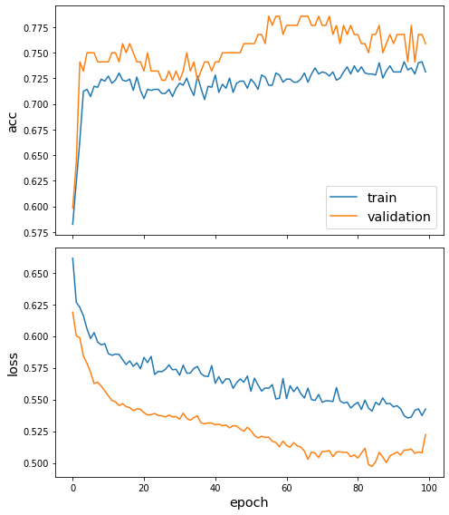
Finally, let us calculate the performance of the trained model on the test data.
[19]:
test_metrics = model.evaluate(test_gen)
print("\nTest Set Metrics:")
for name, val in zip(model.metrics_names, test_metrics):
    print("\t{}: {:0.4f}".format(name, val))
  ['...']
112/112 [==============================] - 0s 1ms/step - loss: 0.5223 - acc: 0.7589

Test Set Metrics:
        loss: 0.5223
        acc: 0.7589
Conclusion
We demonstrated the use of StellarGraph’s DeepGraphCNN implementation for supervised graph classification algorithm. More specifically we showed how to predict whether a chemical compound represented as a graph is an enzyme or not.
Performance is similar to that reported in [1] but a small difference does exist. This difference can be attributed to a small number of factors listed below, - We use a different training scheme, that is a single 90/10 split of the data as opposed to the repeated 10-fold cross validation scheme used in [1]. We use a single fold for ease of exposition. - The experimental evaluation scheme in [1] does not specify some important details such as: the regularisation used for the neural network layers; if a bias term is included; the weight initialization method used; and the batch size.
Execute this notebook:
![]()
![]() Download locally
Download locally
