Execute this notebook: Download locally

Node representation learning with Deep Graph Infomax

This demo demonstrates how to perform unsupervised training of several models using the Deep Graph Infomax algorithm (https://arxiv.org/pdf/1809.10341.pdf) on the CORA dataset:

• GCN (both as a full-batch method, and with the Cluster-GCN training procedure)

• GAT (only as a full-batch method, but the Cluster-GCN training procedure is also supported)

• APPNP (as with GAT, only as a full-batch method, but the Cluster-GCN training procedure is also supported)

• RGCN

• GraphSAGE

• HinSAGE

As with all StellarGraph workflows: first we load the dataset, next we create our data generators, and then we train our model. We then take the embeddings created through unsupervised training and predict the node classes using logistic regression.

See the GCN + Deep Graph Infomax fine-tuning demo for semi-supervised training using Deep Graph Infomax, by fine-tuning the base model for node classification using labelled data.

from stellargraph.mapper import (
    CorruptedGenerator,
    FullBatchNodeGenerator,
    GraphSAGENodeGenerator,
    HinSAGENodeGenerator,
    ClusterNodeGenerator,
)
from stellargraph import StellarGraph
from stellargraph.layer import GCN, DeepGraphInfomax, GraphSAGE, GAT, APPNP, HinSAGE

from stellargraph import datasets
from stellargraph.utils import plot_history

import pandas as pd
from matplotlib import pyplot as plt
from sklearn import model_selection
from sklearn.linear_model import LogisticRegression
from sklearn.manifold import TSNE
from IPython.display import display, HTML

from tensorflow.keras.optimizers import Adam
from tensorflow.keras.callbacks import EarlyStopping
import tensorflow as tf
from tensorflow.keras import Model

(See the “Loading from Pandas” demo for details on how data can be loaded.)

dataset = datasets.Cora()
display(HTML(dataset.description))
G, node_subjects = dataset.load()

The Cora dataset consists of 2708 scientific publications classified into one of seven classes. The citation network consists of 5429 links. Each publication in the dataset is described by a 0/1-valued word vector indicating the absence/presence of the corresponding word from the dictionary. The dictionary consists of 1433 unique words.

Data Generators

Now we create the data generators using CorruptedGenerator (docs). CorruptedGenerator returns shuffled node features along with the regular node features and we train our model to discriminate between the two.

Note that:

• We typically pass all nodes to corrupted_generator.flow because this is an unsupervised task

• We don’t pass targets to corrupted_generator.flow because these are binary labels (true nodes, false nodes) that are created by CorruptedGenerator

fullbatch_generator = FullBatchNodeGenerator(G, sparse=False)
gcn_model = GCN(layer_sizes=[128], activations=["relu"], generator=fullbatch_generator)

corrupted_generator = CorruptedGenerator(fullbatch_generator)
gen = corrupted_generator.flow(G.nodes())

Using GCN (local pooling) filters...

GCN Model Creation and Training

We create and train our DeepGraphInfomax model (docs). Note that the loss used here must always be tf.nn.sigmoid_cross_entropy_with_logits.

infomax = DeepGraphInfomax(gcn_model, corrupted_generator)
x_in, x_out = infomax.in_out_tensors()

model = Model(inputs=x_in, outputs=x_out)
model.compile(loss=tf.nn.sigmoid_cross_entropy_with_logits, optimizer=Adam(lr=1e-3))

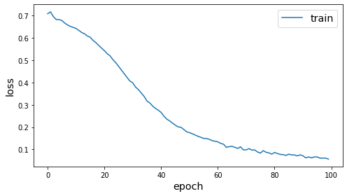
epochs = 100

es = EarlyStopping(monitor="loss", min_delta=0, patience=20)
history = model.fit(gen, epochs=epochs, verbose=0, callbacks=[es])
plot_history(history)

Extracting Embeddings and Logistic Regression

Since we’ve already trained the weights of our base model - GCN in this example - we can simply use base_model.in_out_tensors to obtain the trained node embedding model. Then we use logistic regression on the node embeddings to predict which class the node belongs to.

Note that the results here differ from the paper due to different train/test/val splits.

x_emb_in, x_emb_out = gcn_model.in_out_tensors()

# for full batch models, squeeze out the batch dim (which is 1)
x_out = tf.squeeze(x_emb_out, axis=0)
emb_model = Model(inputs=x_emb_in, outputs=x_out)

train_subjects, test_subjects = model_selection.train_test_split(
    node_subjects, train_size=0.1, test_size=None, stratify=node_subjects
)

test_gen = fullbatch_generator.flow(test_subjects.index)
train_gen = fullbatch_generator.flow(train_subjects.index)

test_embeddings = emb_model.predict(test_gen)
train_embeddings = emb_model.predict(train_gen)

lr = LogisticRegression(multi_class="auto", solver="lbfgs")
lr.fit(train_embeddings, train_subjects)

y_pred = lr.predict(test_embeddings)
gcn_acc = (y_pred == test_subjects).mean()
print(f"Test classification accuracy: {gcn_acc}")

Test classification accuracy: 0.8002461033634126

This accuracy is close to that for training a supervised GCN model end-to-end, suggesting that Deep Graph Infomax is an effective method for unsupervised training.

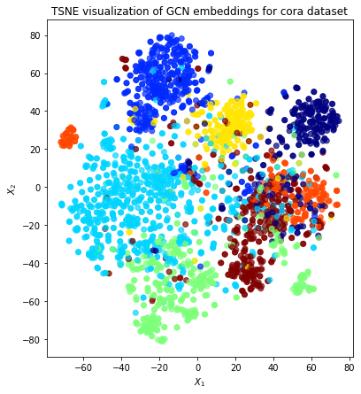
Visualisation with TSNE

Here we visualize the node embeddings with TSNE. As you can see below, the Deep Graph Infomax model produces well separated embeddings using unsupervised training.

all_embeddings = emb_model.predict(fullbatch_generator.flow(G.nodes()))

y = node_subjects.astype("category")
trans = TSNE(n_components=2)
emb_transformed = pd.DataFrame(trans.fit_transform(all_embeddings), index=G.nodes())
emb_transformed["label"] = y

alpha = 0.7

fig, ax = plt.subplots(figsize=(7, 7))
ax.scatter(
    emb_transformed[0],
    emb_transformed[1],
    c=emb_transformed["label"].cat.codes,
    cmap="jet",
    alpha=alpha,
)
ax.set(aspect="equal", xlabel="$X_1$", ylabel="$X_2$")
plt.title("TSNE visualization of GCN embeddings for cora dataset")
plt.show()

Comparing Different Models

Now we run Deep Graph Infomax training for other models. Note that switching between StellarGraph models only requires a few code changes.

def run_deep_graph_infomax(
    base_model, generator, epochs, reorder=lambda sequence, subjects: subjects
):
    corrupted_generator = CorruptedGenerator(generator)
    gen = corrupted_generator.flow(G.nodes())
    infomax = DeepGraphInfomax(base_model, corrupted_generator)

    x_in, x_out = infomax.in_out_tensors()

    model = Model(inputs=x_in, outputs=x_out)
    model.compile(loss=tf.nn.sigmoid_cross_entropy_with_logits, optimizer=Adam(lr=1e-3))
    history = model.fit(gen, epochs=epochs, verbose=0, callbacks=[es])

    x_emb_in, x_emb_out = base_model.in_out_tensors()
    # for full batch models, squeeze out the batch dim (which is 1)
    if generator.num_batch_dims() == 2:
        x_emb_out = tf.squeeze(x_emb_out, axis=0)

    emb_model = Model(inputs=x_emb_in, outputs=x_emb_out)

    test_gen = generator.flow(test_subjects.index)
    train_gen = generator.flow(train_subjects.index)

    test_embeddings = emb_model.predict(test_gen)
    train_embeddings = emb_model.predict(train_gen)

    # some generators yield predictions in a different order to the .flow argument,
    # so we need to get everything lined up correctly
    ordered_test_subjects = reorder(test_gen, test_subjects)
    ordered_train_subjects = reorder(train_gen, train_subjects)

    lr = LogisticRegression(multi_class="auto", solver="lbfgs")
    lr.fit(train_embeddings, ordered_train_subjects)

    y_pred = lr.predict(test_embeddings)
    acc = (y_pred == ordered_test_subjects).mean()

    return acc

Cluster-GCN

Cluster-GCN is a scalable training procedure for that works for several “full batch” models in StellarGraph, including GCN, GAT and APPNP. This example just trains on GCN. The training mechanism breaks the graph into a number of small subgraph “clusters” and trains a single GCN model on these, successively. It is equivalent to full-batch GCN with a single cluster (clusters=1), but with clusters > 1 random clusters (as used here), its performance will be less than GCN. With better clusters, Cluster-GCN performance should be much improved.

(Note: ClusterNodeGenerator can be used with Neo4j for scalable training on large graphs, including unsupervised via Deep Graph Infomax.)

cluster_generator = ClusterNodeGenerator(G, clusters=12, q=4)
cluster_gcn_model = GCN(
    layer_sizes=[128], activations=["relu"], generator=cluster_generator
)


def cluster_reorder(sequence, subjects):
    # shuffle the subjects into the same order as the sequence yield
    return subjects[sequence.node_order]


cluster_gcn_acc = run_deep_graph_infomax(
    cluster_gcn_model, cluster_generator, epochs=epochs, reorder=cluster_reorder
)
print(f"Test classification accuracy: {cluster_gcn_acc}")

Number of clusters 12
0 cluster has size 225
1 cluster has size 225
2 cluster has size 225
3 cluster has size 225
4 cluster has size 225
5 cluster has size 225
6 cluster has size 225
7 cluster has size 225
8 cluster has size 225
9 cluster has size 225
10 cluster has size 225
11 cluster has size 233
Test classification accuracy: 0.6308449548810501

GAT

GAT is a “full batch” model similar to GCN. It can also be trained using both FullBatchNodeGenerator and ClusterNodeGenerator, including for Deep Graph Infomax.

gat_model = GAT(
    layer_sizes=[128], activations=["relu"], generator=fullbatch_generator, attn_heads=8,
)
gat_acc = run_deep_graph_infomax(gat_model, fullbatch_generator, epochs=epochs)

gat_acc
print(f"Test classification accuracy: {gat_acc}")

Test classification accuracy: 0.4716981132075472

APPNP

APPNP is a “full batch” model similar to GCN. It can also be trained using both FullBatchNodeGenerator and ClusterNodeGenerator, including for Deep Graph Infomax.

appnp_model = APPNP(
    layer_sizes=[128], activations=["relu"], generator=fullbatch_generator
)
appnp_acc = run_deep_graph_infomax(appnp_model, fullbatch_generator, epochs=epochs)

print(f"Test classification accuracy: {appnp_acc}")

Test classification accuracy: 0.440935192780968

GraphSAGE

GraphSAGE is a sampling model, different to the models above.

graphsage_generator = GraphSAGENodeGenerator(G, batch_size=1000, num_samples=[5])

graphsage_model = GraphSAGE(
    layer_sizes=[128], activations=["relu"], generator=graphsage_generator
)
graphsage_acc = run_deep_graph_infomax(
    graphsage_model, graphsage_generator, epochs=epochs
)

print(f"Test classification accuracy: {graphsage_acc}")

Test classification accuracy: 0.7210828547990156

Heterogeneous models

Cora is a homogeneous graph, with only one type of node (paper) and one type of edge (type). Models designed for heterogeneous graphs (with more than one of either) can also be applied to homogeneous graphs, but it is not using their additional flexibility.

HinSAGE

HinSAGE is a generalisation of GraphSAGE to heterogeneous graphs that can be trained with Deep Graph Infomax. For homogeneous graphs, it is equivalent to GraphSAGE and it indeed gives similar results.

hinsage_generator = HinSAGENodeGenerator(
    G, batch_size=1000, num_samples=[5], head_node_type="paper"
)

hinsage_model = HinSAGE(
    layer_sizes=[128], activations=["relu"], generator=hinsage_generator
)
hinsage_acc = run_deep_graph_infomax(hinsage_model, hinsage_generator, epochs=epochs)

print(f"Test classification accuracy: {hinsage_acc}")

Test classification accuracy: 0.7042657916324856

RGCN

RGCN is a generalisation of GCN to heterogeneous graphs (with multiple edge types) that can be trained with Deep Graph Infomax. For homogeneous graphs, it is similar to GCN. It normalises the graph’s adjacency matrix in a different manner and so won’t exactly match it.

from stellargraph.mapper import RelationalFullBatchNodeGenerator
from stellargraph.layer import RGCN

rgcn_generator = RelationalFullBatchNodeGenerator(G)

rgcn_model = RGCN(layer_sizes=[128], activations=["relu"], generator=rgcn_generator)

rgcn_acc = run_deep_graph_infomax(rgcn_model, rgcn_generator, epochs=epochs)
print(f"Test classification accuracy: {rgcn_acc}")

Test classification accuracy: 0.7366694011484823

Overall results

The cell below shows the accuracy of each model.

pd.DataFrame(
    [gat_acc, gcn_acc, cluster_gcn_acc, appnp_acc, graphsage_acc, hinsage_acc, rgcn_acc],
    index=["GAT", "GCN", "Cluster-GCN", "APPNP", "GraphSAGE", "HinSAGE", "RGCN"],
    columns=["Accuracy"],
)

	Accuracy
GAT	0.471698
GCN	0.800246
Cluster-GCN	0.630845
APPNP	0.440935
GraphSAGE	0.721083
HinSAGE	0.704266
RGCN	0.736669

Conclusion

This notebook demonstrated how to use the Deep Graph Infomax algorithm to train other algorithms to yield useful embedding vectors for nodes, without supervision. To validate the quality of these vectors, it used logistic regression to perform a supervised node classification task.

See the GCN + Deep Graph Infomax fine-tuning demo for semi-supervised training using Deep Graph Infomax, by fine-tuning the base model for node classification using labelled data.

Execute this notebook: Download locally