Execute this notebook: Download locally

Link prediction with GraphSAGE

In this example, we use our implementation of the GraphSAGE algorithm to build a model that predicts citation links in the Cora dataset (see below). The problem is treated as a supervised link prediction problem on a homogeneous citation network with nodes representing papers (with attributes such as binary keyword indicators and categorical subject) and links corresponding to paper-paper citations.

To address this problem, we build a model with the following architecture. First we build a two-layer GraphSAGE model that takes labeled node pairs (citing-paper -> cited-paper) corresponding to possible citation links, and outputs a pair of node embeddings for the citing-paper and cited-paper nodes of the pair. These embeddings are then fed into a link classification layer, which first applies a binary operator to those node embeddings (e.g., concatenating them) to construct the embedding of the potential link. Thus obtained link embeddings are passed through the dense link classification layer to obtain link predictions - probability for these candidate links to actually exist in the network. The entire model is trained end-to-end by minimizing the loss function of choice (e.g., binary cross-entropy between predicted link probabilities and true link labels, with true/false citation links having labels 1/0) using stochastic gradient descent (SGD) updates of the model parameters, with minibatches of ‘training’ links fed into the model.

import stellargraph as sg
from stellargraph.data import EdgeSplitter
from stellargraph.mapper import GraphSAGELinkGenerator
from stellargraph.layer import GraphSAGE, HinSAGE, link_classification

from tensorflow import keras
from sklearn import preprocessing, feature_extraction, model_selection

from stellargraph import globalvar
from stellargraph import datasets
from IPython.display import display, HTML
%matplotlib inline

Loading the CORA network data

(See the “Loading from Pandas” demo for details on how data can be loaded.)

dataset = datasets.Cora()
display(HTML(dataset.description))
G, _ = dataset.load(subject_as_feature=True)

The Cora dataset consists of 2708 scientific publications classified into one of seven classes. The citation network consists of 5429 links. Each publication in the dataset is described by a 0/1-valued word vector indicating the absence/presence of the corresponding word from the dictionary. The dictionary consists of 1433 unique words.

print(G.info())

StellarGraph: Undirected multigraph
 Nodes: 2708, Edges: 5429

 Node types:
  paper: [2708]
    Features: float32 vector, length 1440
    Edge types: paper-cites->paper

 Edge types:
    paper-cites->paper: [5429]

We aim to train a link prediction model, hence we need to prepare the train and test sets of links and the corresponding graphs with those links removed.

We are going to split our input graph into a train and test graphs using the EdgeSplitter class in stellargraph.data. We will use the train graph for training the model (a binary classifier that, given two nodes, predicts whether a link between these two nodes should exist or not) and the test graph for evaluating the model’s performance on hold out data. Each of these graphs will have the same number of nodes as the input graph, but the number of links will differ (be reduced) as some of the links will be removed during each split and used as the positive samples for training/testing the link prediction classifier.

From the original graph G, extract a randomly sampled subset of test edges (true and false citation links) and the reduced graph G_test with the positive test edges removed:

# Define an edge splitter on the original graph G:
edge_splitter_test = EdgeSplitter(G)

# Randomly sample a fraction p=0.1 of all positive links, and same number of negative links, from G, and obtain the
# reduced graph G_test with the sampled links removed:
G_test, edge_ids_test, edge_labels_test = edge_splitter_test.train_test_split(
    p=0.1, method="global", keep_connected=True
)

** Sampled 542 positive and 542 negative edges. **

The reduced graph G_test, together with the test ground truth set of links (edge_ids_test, edge_labels_test), will be used for testing the model.

Now repeat this procedure to obtain the training data for the model. From the reduced graph G_test, extract a randomly sampled subset of train edges (true and false citation links) and the reduced graph G_train with the positive train edges removed:

# Define an edge splitter on the reduced graph G_test:
edge_splitter_train = EdgeSplitter(G_test)

# Randomly sample a fraction p=0.1 of all positive links, and same number of negative links, from G_test, and obtain the
# reduced graph G_train with the sampled links removed:
G_train, edge_ids_train, edge_labels_train = edge_splitter_train.train_test_split(
    p=0.1, method="global", keep_connected=True
)

** Sampled 488 positive and 488 negative edges. **

G_train, together with the train ground truth set of links (edge_ids_train, edge_labels_train), will be used for training the model.

Summary of G_train and G_test - note that they have the same set of nodes, only differing in their edge sets:

print(G_train.info())

StellarGraph: Undirected multigraph
 Nodes: 2708, Edges: 4399

 Node types:
  paper: [2708]
    Features: float32 vector, length 1440
    Edge types: paper-cites->paper

 Edge types:
    paper-cites->paper: [4399]

print(G_test.info())

StellarGraph: Undirected multigraph
 Nodes: 2708, Edges: 4887

 Node types:
  paper: [2708]
    Features: float32 vector, length 1440
    Edge types: paper-cites->paper

 Edge types:
    paper-cites->paper: [4887]

Next, we create the link generators for sampling and streaming train and test link examples to the model. The link generators essentially “map” pairs of nodes (citing-paper, cited-paper) to the input of GraphSAGE: they take minibatches of node pairs, sample 2-hop subgraphs with (citing-paper, cited-paper) head nodes extracted from those pairs, and feed them, together with the corresponding binary labels indicating whether those pairs represent true or false citation links, to the input layer of the GraphSAGE model, for SGD updates of the model parameters.

Specify the minibatch size (number of node pairs per minibatch) and the number of epochs for training the model:

batch_size = 20
epochs = 20

Specify the sizes of 1- and 2-hop neighbour samples for GraphSAGE. Note that the length of num_samples list defines the number of layers/iterations in the GraphSAGE model. In this example, we are defining a 2-layer GraphSAGE model:

num_samples = [20, 10]

For training we create a generator on the G_train graph, and make an iterator over the training links using the generator’s flow() method. The shuffle=True argument is given to the flow method to improve training.

train_gen = GraphSAGELinkGenerator(G_train, batch_size, num_samples)
train_flow = train_gen.flow(edge_ids_train, edge_labels_train, shuffle=True)

At test time we use the G_test graph and don’t specify the shuffle argument (it defaults to False).

test_gen = GraphSAGELinkGenerator(G_test, batch_size, num_samples)
test_flow = test_gen.flow(edge_ids_test, edge_labels_test)

Build the model: a 2-layer GraphSAGE model acting as node representation learner, with a link classification layer on concatenated (citing-paper, cited-paper) node embeddings.

GraphSAGE part of the model, with hidden layer sizes of 50 for both GraphSAGE layers, a bias term, and no dropout. (Dropout can be switched on by specifying a positive dropout rate, 0 < dropout < 1) Note that the length of layer_sizes list must be equal to the length of num_samples, as len(num_samples) defines the number of hops (layers) in the GraphSAGE model.

layer_sizes = [20, 20]
graphsage = GraphSAGE(
    layer_sizes=layer_sizes, generator=train_gen, bias=True, dropout=0.3
)

# Build the model and expose input and output sockets of graphsage model
# for link prediction
x_inp, x_out = graphsage.in_out_tensors()

Final link classification layer that takes a pair of node embeddings produced by GraphSAGE, applies a binary operator to them to produce the corresponding link embedding (ip for inner product; other options for the binary operator can be seen by running a cell with ?link_classification in it), and passes it through a dense layer:

prediction = link_classification(
    output_dim=1, output_act="relu", edge_embedding_method="ip"
)(x_out)

link_classification: using 'ip' method to combine node embeddings into edge embeddings

Stack the GraphSAGE and prediction layers into a Keras model, and specify the loss

model = keras.Model(inputs=x_inp, outputs=prediction)

model.compile(
    optimizer=keras.optimizers.Adam(lr=1e-3),
    loss=keras.losses.binary_crossentropy,
    metrics=["acc"],
)

Evaluate the initial (untrained) model on the train and test set:

init_train_metrics = model.evaluate(train_flow)
init_test_metrics = model.evaluate(test_flow)

print("\nTrain Set Metrics of the initial (untrained) model:")
for name, val in zip(model.metrics_names, init_train_metrics):
    print("\t{}: {:0.4f}".format(name, val))

print("\nTest Set Metrics of the initial (untrained) model:")
for name, val in zip(model.metrics_names, init_test_metrics):
    print("\t{}: {:0.4f}".format(name, val))

  ['...']
  ['...']

Train Set Metrics of the initial (untrained) model:
        loss: 0.9410
        acc: 0.6250

Test Set Metrics of the initial (untrained) model:
        loss: 0.8328
        acc: 0.6356

Train the model:

history = model.fit(train_flow, epochs=epochs, validation_data=test_flow, verbose=2)

  ['...']
  ['...']
Train for 49 steps, validate for 55 steps
Epoch 1/20
49/49 - 10s - loss: 0.7426 - acc: 0.5379 - val_loss: 0.6572 - val_acc: 0.6181
Epoch 2/20
49/49 - 9s - loss: 0.5920 - acc: 0.7029 - val_loss: 0.5578 - val_acc: 0.6937
Epoch 3/20
49/49 - 9s - loss: 0.4685 - acc: 0.7971 - val_loss: 0.4985 - val_acc: 0.7592
Epoch 4/20
49/49 - 9s - loss: 0.3895 - acc: 0.8576 - val_loss: 0.4869 - val_acc: 0.7648
Epoch 5/20
49/49 - 9s - loss: 0.3421 - acc: 0.8832 - val_loss: 0.4524 - val_acc: 0.7832
Epoch 6/20
49/49 - 9s - loss: 0.3015 - acc: 0.9078 - val_loss: 0.4348 - val_acc: 0.7952
Epoch 7/20
49/49 - 9s - loss: 0.2760 - acc: 0.9027 - val_loss: 0.4401 - val_acc: 0.8072
Epoch 8/20
49/49 - 9s - loss: 0.2543 - acc: 0.9406 - val_loss: 0.4563 - val_acc: 0.7970
Epoch 9/20
49/49 - 10s - loss: 0.2277 - acc: 0.9467 - val_loss: 0.4392 - val_acc: 0.8054
Epoch 10/20
49/49 - 9s - loss: 0.2060 - acc: 0.9549 - val_loss: 0.4476 - val_acc: 0.8063
Epoch 11/20
49/49 - 9s - loss: 0.1916 - acc: 0.9641 - val_loss: 0.4440 - val_acc: 0.8081
Epoch 12/20
49/49 - 9s - loss: 0.1752 - acc: 0.9631 - val_loss: 0.4596 - val_acc: 0.8035
Epoch 13/20
49/49 - 9s - loss: 0.1648 - acc: 0.9734 - val_loss: 0.4625 - val_acc: 0.8164
Epoch 14/20
49/49 - 9s - loss: 0.1562 - acc: 0.9723 - val_loss: 0.4691 - val_acc: 0.8054
Epoch 15/20
49/49 - 9s - loss: 0.1506 - acc: 0.9816 - val_loss: 0.4497 - val_acc: 0.8081
Epoch 16/20
49/49 - 9s - loss: 0.1420 - acc: 0.9785 - val_loss: 0.4657 - val_acc: 0.8127
Epoch 17/20
49/49 - 9s - loss: 0.1264 - acc: 0.9857 - val_loss: 0.4590 - val_acc: 0.8090
Epoch 18/20
49/49 - 9s - loss: 0.1314 - acc: 0.9826 - val_loss: 0.4655 - val_acc: 0.8035
Epoch 19/20
49/49 - 9s - loss: 0.1234 - acc: 0.9877 - val_loss: 0.5028 - val_acc: 0.8035
Epoch 20/20
49/49 - 9s - loss: 0.1077 - acc: 0.9939 - val_loss: 0.4817 - val_acc: 0.7989

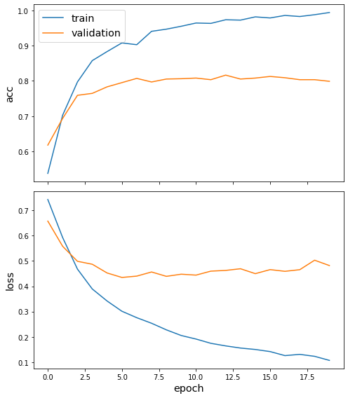
Plot the training history:

sg.utils.plot_history(history)

Evaluate the trained model on test citation links:

train_metrics = model.evaluate(train_flow)
test_metrics = model.evaluate(test_flow)

print("\nTrain Set Metrics of the trained model:")
for name, val in zip(model.metrics_names, train_metrics):
    print("\t{}: {:0.4f}".format(name, val))

print("\nTest Set Metrics of the trained model:")
for name, val in zip(model.metrics_names, test_metrics):
    print("\t{}: {:0.4f}".format(name, val))

  ['...']
  ['...']

Train Set Metrics of the trained model:
        loss: 0.0544
        acc: 0.9959

Test Set Metrics of the trained model:
        loss: 0.4899
        acc: 0.7970

Execute this notebook: Download locally