Execute this notebook: Download locally

Knowledge graph link prediction with DistMult

This notebook reproduces the experiments done in the paper that introduced the DistMult algorithm: Embedding Entities and Relations for Learning and Inference in Knowledge Bases, Bishan Yang, Scott Wen-tau Yih, Xiaodong He, Jianfeng Gao and Li Deng, ICLR 2015. https://arxiv.org/pdf/1412.6575

In table 2, the paper reports 2 metrics measured on the WN18 and FB15K datasets (and FB15k-401): MRR (mean reciprocal rank) and Hits at 10. These are computed as “filtered”, where known edges (in the train, test or validation sets) are ignored when computing ranks.

from stellargraph import datasets, utils
from tensorflow.keras import callbacks, optimizers, losses, metrics, regularizers, Model
import numpy as np
import pandas as pd

from stellargraph.mapper import KGTripleGenerator
from stellargraph.layer import DistMult

from IPython.display import HTML

Initialisation

We need to set up our model parameters, like the number of epochs to train for, and the dimension of the embedding vectors we compute for each node and for each edge type.

The evaluation is performed in three steps:

1. Load the data

2. Train a model

3. Evaluate the model

On pages 4 and 5, the paper describes their implementation details. The paper says that it uses:

• the AdaGrad optimiser for 100 (for FB15k) or 300 epochs (for WN18)

• an embedding dimension of 100

• samples 2 corrupted edges per true edge

• unit normalization of each entity embedding vector after each epoch: this is not currently supported by TensorFlow (#33755), and so may explain the slightly poorer MRR metrics on WN18

epochs = 300
embedding_dimension = 100
negative_samples = 2

WN18

The paper uses the WN18 and FB15k datasets for validation. These datasets are not good for evaluating algorithms because they contain “inverse relations”, where (s, r1, o) implies (o, r2, s) for a pair of relation types r1 and r2 (for instance, _hyponym (“is more specific than”) and _hypernym (“is more general than”) in WN18), however, they work fine to demonstrate StellarGraph’s functionality, and are appropriate to compare against the published results.

Load the data

The dataset comes with a defined train, test and validation split, each consisting of subject, relation, object triples. We can load a StellarGraph object with all of the triples, as well as the individual splits as Pandas DataFrames, using the load method of the WN18 dataset.

(See the “Loading from Pandas” demo for details on how data can be loaded.)

wn18 = datasets.WN18()
display(HTML(wn18.description))
wn18_graph, wn18_train, wn18_test, wn18_valid = wn18.load()

The WN18 dataset consists of triplets from WordNet 3.0 (http://wordnet.princeton.edu). There are 40,943 synsets and 18 relation types among them. The training set contains 141442 triplets, the validation set 5000 and the test set 5000. Antoine Bordes, Xavier Glorot, Jason Weston and Yoshua Bengio “A Semantic Matching Energy Function for Learning with Multi-relational Data” (2014). Note: this dataset contains many inverse relations, and so should only be used to compare against published results. Prefer WN18RR. See: Kristina Toutanova and Danqi Chen “Observed versus latent features for knowledge base and text inference” (2015), and Dettmers, Tim, Pasquale Minervini, Pontus Stenetorp and Sebastian Riedel “Convolutional 2D Knowledge Graph Embeddings” (2017).

print(wn18_graph.info())

StellarDiGraph: Directed multigraph
 Nodes: 40943, Edges: 151442

 Node types:
  default: [40943]
    Features: none
    Edge types: default-_also_see->default, default-_derivationally_related_form->default, default-_has_part->default, default-_hypernym->default, default-_hyponym->default, ... (13 more)

 Edge types:
    default-_hyponym->default: [37221]
    default-_hypernym->default: [37221]
    default-_derivationally_related_form->default: [31867]
    default-_member_meronym->default: [7928]
    default-_member_holonym->default: [7928]
    default-_part_of->default: [5148]
    default-_has_part->default: [5142]
    default-_member_of_domain_topic->default: [3341]
    default-_synset_domain_topic_of->default: [3335]
    default-_instance_hyponym->default: [3150]
    default-_instance_hypernym->default: [3150]
    default-_also_see->default: [1396]
    default-_verb_group->default: [1220]
    default-_member_of_domain_region->default: [983]
    default-_synset_domain_region_of->default: [982]
    default-_member_of_domain_usage->default: [675]
    default-_synset_domain_usage_of->default: [669]
    default-_similar_to->default: [86]

Train a model

The DistMult algorithm consists of some embedding layers and a scoring layer, but the DistMult object means these details are invisible to us. The DistMult model consumes “knowledge-graph triples”, which can be produced in the appropriate format using KGTripleGenerator.

wn18_gen = KGTripleGenerator(
    wn18_graph, batch_size=len(wn18_train) // 10  # ~10 batches per epoch
)

wn18_distmult = DistMult(
    wn18_gen,
    embedding_dimension=embedding_dimension,
    embeddings_regularizer=regularizers.l2(1e-7),
)

wn18_inp, wn18_out = wn18_distmult.in_out_tensors()

wn18_model = Model(inputs=wn18_inp, outputs=wn18_out)

wn18_model.compile(
    optimizer=optimizers.Adam(lr=0.001),
    loss=losses.BinaryCrossentropy(from_logits=True),
    metrics=[metrics.BinaryAccuracy(threshold=0.0)],
)

Inputs for training are produced by calling the KGTripleGenerator.flow method, this takes a dataframe with source, label and target columns, where each row is a true edge in the knowledge graph. The negative_samples parameter controls how many random edges are created for each positive edge to use as negative examples for training.

wn18_train_gen = wn18_gen.flow(
    wn18_train, negative_samples=negative_samples, shuffle=True
)
wn18_valid_gen = wn18_gen.flow(wn18_valid, negative_samples=negative_samples)

wn18_es = callbacks.EarlyStopping(monitor="val_loss", patience=50)
wn18_history = wn18_model.fit(
    wn18_train_gen,
    validation_data=wn18_valid_gen,
    epochs=epochs,
    callbacks=[wn18_es],
    verbose=0,
)

  ['...']
  ['...']

utils.plot_history(wn18_history)

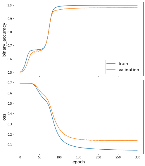
Evaluate the model

We’ve now trained a model, so we can apply the evaluation procedure from the paper to it. This is done by taking each test edge E = (s, r, o), and scoring it against all mutations (s, r, n) and (n, r, o) for every node n in the graph, that is, doing a prediction for every one of these edges similar to E. The “raw” rank is the number of mutated edges that have a higher predicted score than the true E.

The DistMult paper uses only 10 batches per epoch, which results in large batch sizes: ~15 thousand edges per batch for WN18, and ~60 thousand edges per batch for the FB15k dataset below. Evaluation with rank_edges_against_all_nodes uses bulk operations for efficient reasons, at the cost of memory usage proportional to O(batch size * number of nodes); a more moderate batch size gives similar performance without using large amounts of memory. We can swap the batch size by creating a new generator.

wn18_smaller_gen = KGTripleGenerator(wn18_graph, batch_size=5000)

wn18_raw_ranks, wn18_filtered_ranks = wn18_distmult.rank_edges_against_all_nodes(
    wn18_smaller_gen.flow(wn18_test), wn18_graph
)

# helper function to compute metrics from an array of ranks
def results_as_dataframe(mrr, hits_at_10):
    return pd.DataFrame(
        [(mrr, hits_at_10)], columns=["mrr", "hits at 10"], index=["filtered"],
    )


def summarise(ranks):
    return results_as_dataframe(np.mean(1 / ranks), np.mean(ranks <= 10))

summarise(wn18_filtered_ranks)

	mrr	hits at 10
filtered	0.709954	0.9303

For comparison, Table 2 in the paper gives the following results for WN18. All of the numbers are similar:

results_as_dataframe(0.83, 0.942)

	mrr	hits at 10
filtered	0.83	0.942

FB15k

Now that we know the process, we can apply the model on the FB15k dataset in the same way.

Loading the data

fb15k = datasets.FB15k()
display(HTML(fb15k.description))
fb15k_graph, fb15k_train, fb15k_test, fb15k_valid = fb15k.load()

This FREEBASE FB15k DATA consists of a collection of triplets (synset, relation_type, triplet)extracted from Freebase (http://www.freebase.com). There are 14,951 mids and 1,345 relation types among them. The training set contains 483142 triplets, the validation set 50000 and the test set 59071. Antoine Bordes, Nicolas Usunier, Alberto Garcia-Durán, Jason Weston and Oksana Yakhnenko “Translating Embeddings for Modeling Multi-relational Data” (2013). Note: this dataset contains many inverse relations, and so should only be used to compare against published results. Prefer FB15k_237. See: Kristina Toutanova and Danqi Chen “Observed versus latent features for knowledge base and text inference” (2015), and Dettmers, Tim, Pasquale Minervini, Pontus Stenetorp and Sebastian Riedel “Convolutional 2D Knowledge Graph Embeddings” (2017).

print(fb15k_graph.info())

StellarDiGraph: Directed multigraph
 Nodes: 14951, Edges: 592213

 Node types:
  default: [14951]
    Features: none
    Edge types: default-/american_football/football_coach/coaching_history./american_football/football_historical_coach_position/position->default, default-/american_football/football_coach/coaching_history./american_football/football_historical_coach_position/team->default, default-/american_football/football_coach_position/coaches_holding_this_position./american_football/football_historical_coach_position/coach->default, default-/american_football/football_coach_position/coaches_holding_this_position./american_football/football_historical_coach_position/team->default, default-/american_football/football_player/current_team./american_football/football_roster_position/position->default, ... (1340 more)

 Edge types:
    default-/award/award_nominee/award_nominations./award/award_nomination/award_nominee->default: [19764]
    default-/film/film/release_date_s./film/film_regional_release_date/film_release_region->default: [15837]
    default-/award/award_nominee/award_nominations./award/award_nomination/award->default: [14921]
    default-/award/award_category/nominees./award/award_nomination/award_nominee->default: [14921]
    default-/people/profession/people_with_this_profession->default: [14220]
    default-/people/person/profession->default: [14220]
    default-/film/film/starring./film/performance/actor->default: [11638]
    default-/film/actor/film./film/performance/film->default: [11638]
    default-/award/award_nominated_work/award_nominations./award/award_nomination/award->default: [11594]
    default-/award/award_category/nominees./award/award_nomination/nominated_for->default: [11594]
    default-/award/award_winner/awards_won./award/award_honor/award_winner->default: [10378]
    default-/film/film_genre/films_in_this_genre->default: [8946]
    default-/film/film/genre->default: [8946]
    default-/award/award_nominee/award_nominations./award/award_nomination/nominated_for->default: [7632]
    default-/award/award_nominated_work/award_nominations./award/award_nomination/award_nominee->default: [7632]
    default-/film/film_job/films_with_this_crew_job./film/film_crew_gig/film->default: [7400]
    default-/film/film/other_crew./film/film_crew_gig/film_crew_role->default: [7400]
    default-/common/topic/webpage./common/webpage/category->default: [7232]
    default-/common/annotation_category/annotations./common/webpage/topic->default: [7232]
    default-/music/genre/artists->default: [7229]
    ... (1325 more)

Train a model

fb15k_gen = KGTripleGenerator(
    fb15k_graph, batch_size=len(fb15k_train) // 10  # ~100 batches per epoch
)

fb15k_distmult = DistMult(
    fb15k_gen,
    embedding_dimension=embedding_dimension,
    embeddings_regularizer=regularizers.l2(1e-8),
)

fb15k_inp, fb15k_out = fb15k_distmult.in_out_tensors()

fb15k_model = Model(inputs=fb15k_inp, outputs=fb15k_out)
fb15k_model.compile(
    optimizer=optimizers.Adam(lr=0.001),
    loss=losses.BinaryCrossentropy(from_logits=True),
    metrics=[metrics.BinaryAccuracy(threshold=0.0)],
)

fb15k_train_gen = fb15k_gen.flow(
    fb15k_train, negative_samples=negative_samples, shuffle=True
)
fb15k_valid_gen = fb15k_gen.flow(fb15k_valid, negative_samples=negative_samples)

fb15k_es = callbacks.EarlyStopping(monitor="val_loss", patience=50)
fb15k_history = fb15k_model.fit(
    fb15k_train_gen,
    validation_data=fb15k_valid_gen,
    epochs=epochs,
    callbacks=[fb15k_es],
    verbose=0,
)

  ['...']
  ['...']

utils.plot_history(fb15k_history)

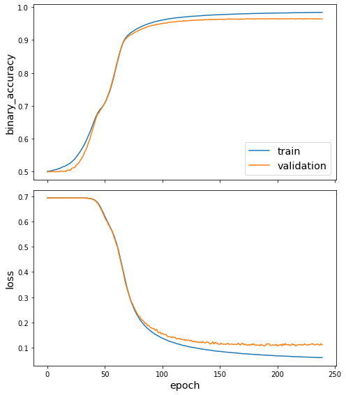
Evaluate the model

fb15k_smaller_gen = KGTripleGenerator(fb15k_graph, batch_size=5000)

fb15k_raw_ranks, fb15k_filtered_ranks = fb15k_distmult.rank_edges_against_all_nodes(
    fb15k_smaller_gen.flow(fb15k_test), fb15k_graph
)

summarise(fb15k_filtered_ranks)

	mrr	hits at 10
filtered	0.33919	0.579582

For comparison, Table 2 in the paper gives the following results for FB15k:

results_as_dataframe(0.35, 0.577)

	mrr	hits at 10
filtered	0.35	0.577

Execute this notebook: Download locally