Execute this notebook:
![]()
![]() Download locally
Download locally
Interpreting nodes and edges with saliency maps in GAT
This demo shows how to use integrated gradients in graph attention networks to obtain accurate importance estimations for both the nodes and edges. The notebook consists of three parts:
setting up the node classification problem for Cora citation network training and evaluating a GAT model for node classification calculating node and edge importances for model’s predictions of query (“target”) nodes.
[3]:
import networkx as nx
import pandas as pd
import numpy as np
from scipy import stats
import os
import time
import sys
import stellargraph as sg
from copy import deepcopy


from stellargraph.mapper import FullBatchNodeGenerator
from stellargraph.layer import GAT, GraphAttention

from tensorflow.keras import layers, optimizers, losses, metrics, models, Model
from sklearn import preprocessing, feature_extraction, model_selection
from tensorflow.keras import backend as K
import matplotlib.pyplot as plt
from stellargraph import datasets
from IPython.display import display, HTML
%matplotlib inline
Loading the CORA network
(See the “Loading from Pandas” demo for details on how data can be loaded.)
[4]:
dataset = datasets.Cora()
display(HTML(dataset.description))
G, subjects = dataset.load()
[5]:
print(G.info())
StellarGraph: Undirected multigraph
 Nodes: 2708, Edges: 5429

 Node types:
  paper: [2708]
    Features: float32 vector, length 1433
    Edge types: paper-cites->paper

 Edge types:
    paper-cites->paper: [5429]
Splitting the data
For machine learning we want to take a subset of the nodes for training, and use the rest for validation and testing. We’ll use scikit-learn again to do this.
Here we’re taking 140 node labels for training, 500 for validation, and the rest for testing.
[6]:
train_subjects, test_subjects = model_selection.train_test_split(
    subjects, train_size=140, test_size=None, stratify=subjects
)
val_subjects, test_subjects = model_selection.train_test_split(
    test_subjects, train_size=500, test_size=None, stratify=test_subjects
)
[7]:
from collections import Counter

Counter(train_subjects)
[7]:
Counter({'Theory': 18,
         'Neural_Networks': 42,
         'Genetic_Algorithms': 22,
         'Case_Based': 16,
         'Rule_Learning': 9,
         'Probabilistic_Methods': 22,
         'Reinforcement_Learning': 11})
Converting to numeric arrays
For our categorical target, we will use one-hot vectors that will be fed into a soft-max Keras layer during training. To do this conversion …
[8]:
target_encoding = preprocessing.LabelBinarizer()

train_targets = target_encoding.fit_transform(train_subjects)
val_targets = target_encoding.transform(val_subjects)
test_targets = target_encoding.transform(test_subjects)

all_targets = target_encoding.transform(subjects)
Creating the GAT model in Keras
To feed data from the graph to the Keras model we need a generator. Since GAT is a full-batch model, we use the FullBatchNodeGenerator class to feed node features and graph adjacency matrix to the model.
[9]:
generator = FullBatchNodeGenerator(G, method="gat", sparse=False)
For training we map only the training nodes returned from our splitter and the target values.
[10]:
train_gen = generator.flow(train_subjects.index, train_targets)
Now we can specify our machine learning model, we need a few more parameters for this:
the
layer_sizesis a list of hidden feature sizes of each layer in the model. In this example we use two GAT layers with 8-dimensional hidden node features at each layer.attn_headsis the number of attention heads in all but the last GAT layer in the modelactivationsis a list of activations applied to each layer’s outputArguments such as
bias,in_dropout,attn_dropoutare internal parameters of the model, execute?GATfor details.
To follow the GAT model architecture used for Cora dataset in the original paper [Graph Attention Networks. P. Veličković et al. ICLR 2018 https://arxiv.org/abs/1803.07294], let’s build a 2-layer GAT model, with the second layer being the classifier that predicts paper subject: it thus should have the output size of train_targets.shape[1] (7 subjects) and a softmax activation.
[11]:
gat = GAT(
    layer_sizes=[8, train_targets.shape[1]],
    attn_heads=8,
    generator=generator,
    bias=True,
    in_dropout=0,
    attn_dropout=0,
    activations=["elu", "softmax"],
    normalize=None,
    saliency_map_support=True,
)
[12]:
# Expose the input and output tensors of the GAT model for node prediction, via GAT.in_out_tensors() method:
x_inp, predictions = gat.in_out_tensors()
Training the model
Now let’s create the actual Keras model with the input tensors x_inp and output tensors being the predictions predictions from the final dense layer
[13]:
model = Model(inputs=x_inp, outputs=predictions)
model.compile(
    optimizer=optimizers.Adam(lr=0.005),
    loss=losses.categorical_crossentropy,
    weighted_metrics=["acc"],
)
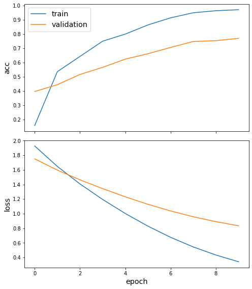
Train the model, keeping track of its loss and accuracy on the training set, and its generalisation performance on the validation set (we need to create another generator over the validation data for this)
[14]:
val_gen = generator.flow(val_subjects.index, val_targets)
Train the model
[15]:
N = G.number_of_nodes()
history = model.fit(
    train_gen, validation_data=val_gen, shuffle=False, epochs=10, verbose=2
)
Epoch 1/10
1/1 - 9s - loss: 1.9274 - acc: 0.1571 - val_loss: 1.7515 - val_acc: 0.3960
Epoch 2/10
1/1 - 2s - loss: 1.6477 - acc: 0.5357 - val_loss: 1.5972 - val_acc: 0.4440
Epoch 3/10
1/1 - 2s - loss: 1.4080 - acc: 0.6429 - val_loss: 1.4644 - val_acc: 0.5160
Epoch 4/10
1/1 - 2s - loss: 1.1955 - acc: 0.7500 - val_loss: 1.3436 - val_acc: 0.5660
Epoch 5/10
1/1 - 2s - loss: 1.0033 - acc: 0.8000 - val_loss: 1.2316 - val_acc: 0.6240
Epoch 6/10
1/1 - 2s - loss: 0.8298 - acc: 0.8643 - val_loss: 1.1291 - val_acc: 0.6620
Epoch 7/10
1/1 - 2s - loss: 0.6770 - acc: 0.9143 - val_loss: 1.0381 - val_acc: 0.7060
Epoch 8/10
1/1 - 2s - loss: 0.5456 - acc: 0.9500 - val_loss: 0.9591 - val_acc: 0.7480
Epoch 9/10
1/1 - 2s - loss: 0.4348 - acc: 0.9643 - val_loss: 0.8916 - val_acc: 0.7540
Epoch 10/10
1/1 - 2s - loss: 0.3428 - acc: 0.9714 - val_loss: 0.8356 - val_acc: 0.7700
[16]:
sg.utils.plot_history(history)
Evaluate the trained model on the test set
[17]:
test_gen = generator.flow(test_subjects.index, test_targets)

test_metrics = model.evaluate(test_gen)
print("\nTest Set Metrics:")
for name, val in zip(model.metrics_names, test_metrics):
    print("\t{}: {:0.4f}".format(name, val))
Test Set Metrics:
        loss: 0.7781
        acc: 0.7955
Check serialization
[18]:
# Save model
model_json = model.to_json()
model_weights = model.get_weights()
[19]:
# Load model from json & set all weights
model2 = models.model_from_json(model_json, custom_objects=sg.custom_keras_layers)
model2.set_weights(model_weights)
model2_weights = model2.get_weights()
[20]:
pred2 = model2.predict(test_gen)
pred1 = model.predict(test_gen)
print(np.allclose(pred1, pred2))
True
Node and link importance via saliency maps
Now we define the importances of node features, nodes, and links in the target node’s neighbourhood (ego-net), and evaluate them using our library.
Node feature importance: given a target node \(t\) and the model’s prediction of \(t\)’s class, for each node \(v\) in its ego-net, feature importance of feature \(f\) for node \(v\) is defined as the change in the target node’s predicted score \(s(c)\) for the winning class \(c\) if feature \(f\) of node \(v\) is perturbed.
The overall node importance for node \(v\) is defined here as the sum of all feature importances for node \(v\), i.e., it is the amount by which the target node’s predicted score \(s(c)\) would change if we set all features of node \(v\) to zeros.
Link importance for link \(e=(u, v)\) is defined as the change in target node \(t\)’s predicted score \(s(c)\) if the link \(e\) is removed from the graph. Links with high importance (positive or negative) affect the target node prediction more than links with low importance.
Node and link importances can be used to assess the role of neighbour nodes and links in model’s predictions for the node(s) of interest (the target nodes). For datasets like CORA-ML, the features and edges are binary, vanilla gradients may not perform well so we use integrated gradients to compute them (https://arxiv.org/pdf/1703.01365.pdf).
[21]:
from stellargraph.interpretability.saliency_maps import IntegratedGradientsGAT
from stellargraph.interpretability.saliency_maps import GradientSaliencyGAT
Select the target node whose prediction is to be interpreted.
[22]:
graph_nodes = list(G.nodes())
all_gen = generator.flow(graph_nodes)
target_nid = 1109199
target_idx = graph_nodes.index(target_nid)
target_gen = generator.flow([target_nid])
Node id of the target node:
[23]:
y_true = all_targets[target_idx] # true class of the target node
Extract adjacency matrix and feature matrix
[24]:
y_pred = model.predict(target_gen).squeeze()
class_of_interest = np.argmax(y_pred)
print(
    "target node id: {}, \ntrue label: {}, \npredicted label: {}".format(
        target_nid, y_true, y_pred.round(2)
    )
)
target node id: 1109199,
true label: [0 1 0 0 0 0 0],
predicted label: [0.05 0.75 0.06 0.02 0.06 0.02 0.03]
Get the node feature importance by using integrated gradients
[25]:
int_grad_saliency = IntegratedGradientsGAT(model, train_gen, generator.node_list)
saliency = GradientSaliencyGAT(model, train_gen)
Get the ego network of the target node.
[26]:
G_ego = nx.ego_graph(G.to_networkx(), target_nid, radius=len(gat.activations))
Compute the link importance by integrated gradients.
[27]:
integrate_link_importance = int_grad_saliency.get_link_importance(
    target_nid, class_of_interest, steps=25
)
print("integrated_link_mask.shape = {}".format(integrate_link_importance.shape))
To change all layers to have dtype float64 by default, call `tf.keras.backend.set_floatx('float64')`. To change just this layer, pass dtype='float64' to the layer constructor. If you are the author of this layer, you can disable autocasting by passing autocast=False to the base Layer constructor.

integrated_link_mask.shape = (2708, 2708)
[28]:
integrated_node_importance = int_grad_saliency.get_node_importance(
    target_nid, class_of_interest, steps=25
)
print("\nintegrated_node_importance", integrated_node_importance.round(2))
print(
    "integrated self-importance of target node {}: {}".format(
        target_nid, integrated_node_importance[target_idx].round(2)
    )
)
print(
    "\nEgo net of target node {} has {} nodes".format(target_nid, G_ego.number_of_nodes())
)
print(
    "Number of non-zero elements in integrated_node_importance: {}".format(
        np.count_nonzero(integrated_node_importance)
    )
)
To change all layers to have dtype float64 by default, call `tf.keras.backend.set_floatx('float64')`. To change just this layer, pass dtype='float64' to the layer constructor. If you are the author of this layer, you can disable autocasting by passing autocast=False to the base Layer constructor.


integrated_node_importance [0. 0. 0. ... 0. 0. 0.]
integrated self-importance of target node 1109199: 0.47

Ego net of target node 1109199 has 202 nodes
Number of non-zero elements in integrated_node_importance: 212
Get the ranks of the edge importance values.
[29]:
sorted_indices = np.argsort(integrate_link_importance.flatten().reshape(-1))
sorted_indices = np.array(sorted_indices)
integrated_link_importance_rank = [(int(k / N), k % N) for k in sorted_indices[::-1]]
[30]:
topk = 10
print(
    "Top {} most important links by integrated gradients are {}".format(
        topk, integrated_link_importance_rank[:topk]
    )
)
# print('Top {} most important links by integrated gradients (for potential edges) are {}'.format(topk, integrated_link_importance_rank_add[-topk:]))
Top 10 most important links by integrated gradients are [(1544, 163), (1206, 163), (1544, 1206), (1206, 789), (163, 219), (163, 163), (566, 294), (566, 733), (163, 1136), (163, 1098)]
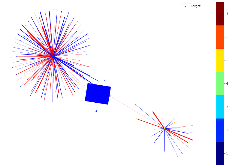
In the following, we plot the link and node importance (computed by integrated gradients) of the nodes within the ego graph of the target node.
For nodes, the shape of the node indicates the positive/negative importance the node has. ‘round’ nodes have positive importance while ‘diamond’ nodes have negative importance. The size of the node indicates the value of the importance, e.g., a large diamond node has higher negative importance.
For links, the color of the link indicates the positive/negative importance the link has. ‘red’ links have positive importance while ‘blue’ links have negative importance. The width of the link indicates the value of the importance, e.g., a thicker blue link has higher negative importance.
[31]:
nx.set_node_attributes(G_ego, values={x[0]: {"subject": x[1]} for x in subjects.items()})
[32]:
node_size_factor = 1e2
link_width_factor = 4

nodes = list(G_ego.nodes())
colors = pd.DataFrame(
    [v[1]["subject"] for v in G_ego.nodes(data=True)], index=nodes, columns=["subject"]
)
colors = np.argmax(target_encoding.transform(colors), axis=1) + 1

fig, ax = plt.subplots(1, 1, figsize=(15, 10))
pos = nx.spring_layout(G_ego)
# Draw ego as large and red
node_sizes = [integrated_node_importance[graph_nodes.index(k)] for k in nodes]
node_shapes = [
    "o" if integrated_node_importance[graph_nodes.index(k)] > 0 else "d" for k in nodes
]
positive_colors, negative_colors = [], []
positive_node_sizes, negative_node_sizes = [], []
positive_nodes, negative_nodes = [], []
# node_size_sclae is used for better visualization of nodes
node_size_scale = node_size_factor / np.max(node_sizes)
for k in range(len(node_shapes)):
    if list(nodes)[k] == target_nid:
        continue
    if node_shapes[k] == "o":
        positive_colors.append(colors[k])
        positive_nodes.append(list(nodes)[k])
        positive_node_sizes.append(node_size_scale * node_sizes[k])

    else:
        negative_colors.append(colors[k])
        negative_nodes.append(list(nodes)[k])
        negative_node_sizes.append(node_size_scale * abs(node_sizes[k]))

cmap = plt.get_cmap("jet", np.max(colors) - np.min(colors) + 1)
nc = nx.draw_networkx_nodes(
    G_ego,
    pos,
    nodelist=positive_nodes,
    node_color=positive_colors,
    cmap=cmap,
    node_size=positive_node_sizes,
    vmin=np.min(colors) - 0.5,
    vmax=np.max(colors) + 0.5,
    node_shape="o",
)
nc = nx.draw_networkx_nodes(
    G_ego,
    pos,
    nodelist=negative_nodes,
    node_color=negative_colors,
    cmap=cmap,
    node_size=negative_node_sizes,
    vmin=np.min(colors) - 0.5,
    vmax=np.max(colors) + 0.5,
    node_shape="d",
)
# Draw the target node as a large star colored by its true subject
nx.draw_networkx_nodes(
    G_ego,
    pos,
    nodelist=[target_nid],
    node_size=50 * abs(node_sizes[nodes.index(target_nid)]),
    node_shape="*",
    node_color=[colors[nodes.index(target_nid)]],
    cmap=cmap,
    vmin=np.min(colors) - 0.5,
    vmax=np.max(colors) + 0.5,
    label="Target",
)

edges = G_ego.edges()
# link_width_scale is used for better visualization of links
weights = [
    integrate_link_importance[graph_nodes.index(u), graph_nodes.index(v)]
    for u, v in edges
]
link_width_scale = link_width_factor / np.max(weights)
edge_colors = [
    "red"
    if integrate_link_importance[graph_nodes.index(u), graph_nodes.index(v)] > 0
    else "blue"
    for u, v in edges
]

ec = nx.draw_networkx_edges(
    G_ego, pos, edge_color=edge_colors, width=[link_width_scale * w for w in weights]
)
plt.legend()
plt.colorbar(nc, ticks=np.arange(np.min(colors), np.max(colors) + 1))
plt.axis("off")
plt.show()
We then remove the node or edge in the ego graph one by one and check how the prediction changes. By doing so, we can obtain the ground truth importance of the nodes and edges. Comparing the following figure and the above one can show the effectiveness of integrated gradients as the importance approximations are relatively consistent with the ground truth.
[33]:
[X, _, A], y_true_all = all_gen[0]
N = A.shape[-1]
X_bk = deepcopy(X)
edges = [(graph_nodes.index(u), graph_nodes.index(v)) for u, v in G_ego.edges()]
nodes_idx = [graph_nodes.index(v) for v in nodes]
selected_nodes = np.array([[target_idx]], dtype="int32")
clean_prediction = model.predict([X, selected_nodes, A]).squeeze()
predict_label = np.argmax(clean_prediction)
groud_truth_edge_importance = np.zeros((N, N), dtype="float")
groud_truth_node_importance = []

for node in nodes_idx:
    if node == target_idx:
        groud_truth_node_importance.append(0)
        continue
    X = deepcopy(X_bk)
    # we set all the features of the node to zero to check the ground truth node importance.
    X[0, node, :] = 0
    predict_after_perturb = model.predict([X, selected_nodes, A]).squeeze()
    prediction_change = (
        clean_prediction[predict_label] - predict_after_perturb[predict_label]
    )
    groud_truth_node_importance.append(prediction_change)

node_shapes = [
    "o" if groud_truth_node_importance[k] > 0 else "d" for k in range(len(nodes))
]
positive_colors, negative_colors = [], []
positive_node_sizes, negative_node_sizes = [], []
positive_nodes, negative_nodes = [], []
# node_size_scale is used for better visulization of nodes
node_size_scale = node_size_factor / max(groud_truth_node_importance)

for k in range(len(node_shapes)):
    if nodes_idx[k] == target_idx:
        continue
    if node_shapes[k] == "o":
        positive_colors.append(colors[k])
        positive_nodes.append(graph_nodes[nodes_idx[k]])
        positive_node_sizes.append(node_size_scale * groud_truth_node_importance[k])
    else:
        negative_colors.append(colors[k])
        negative_nodes.append(graph_nodes[nodes_idx[k]])
        negative_node_sizes.append(node_size_scale * abs(groud_truth_node_importance[k]))

X = deepcopy(X_bk)
for edge in edges:
    original_val = A[0, edge[0], edge[1]]
    if original_val == 0:
        continue
    # we set the weight of a given edge to zero to check the ground truth link importance
    A[0, edge[0], edge[1]] = 0
    predict_after_perturb = model.predict([X, selected_nodes, A]).squeeze()
    groud_truth_edge_importance[edge[0], edge[1]] = (
        predict_after_perturb[predict_label] - clean_prediction[predict_label]
    ) / (0 - 1)
    A[0, edge[0], edge[1]] = original_val
#     print(groud_truth_edge_importance[edge[0], edge[1]])

fig, ax = plt.subplots(1, 1, figsize=(15, 10))
cmap = plt.get_cmap("jet", np.max(colors) - np.min(colors) + 1)
# Draw the target node as a large star colored by its true subject
nx.draw_networkx_nodes(
    G_ego,
    pos,
    nodelist=[target_nid],
    node_size=50 * abs(node_sizes[nodes_idx.index(target_idx)]),
    node_color=[colors[nodes_idx.index(target_idx)]],
    cmap=cmap,
    node_shape="*",
    vmin=np.min(colors) - 0.5,
    vmax=np.max(colors) + 0.5,
    label="Target",
)
# Draw the ego net
nc = nx.draw_networkx_nodes(
    G_ego,
    pos,
    nodelist=positive_nodes,
    node_color=positive_colors,
    cmap=cmap,
    node_size=positive_node_sizes,
    vmin=np.min(colors) - 0.5,
    vmax=np.max(colors) + 0.5,
    node_shape="o",
)
nc = nx.draw_networkx_nodes(
    G_ego,
    pos,
    nodelist=negative_nodes,
    node_color=negative_colors,
    cmap=cmap,
    node_size=negative_node_sizes,
    vmin=np.min(colors) - 0.5,
    vmax=np.max(colors) + 0.5,
    node_shape="d",
)
edges = G_ego.edges()
# link_width_scale is used for better visulization of links
link_width_scale = link_width_factor / np.max(groud_truth_edge_importance)
weights = [
    link_width_scale
    * groud_truth_edge_importance[graph_nodes.index(u), graph_nodes.index(v)]
    for u, v in edges
]

edge_colors = [
    "red"
    if groud_truth_edge_importance[graph_nodes.index(u), graph_nodes.index(v)] > 0
    else "blue"
    for u, v in edges
]

ec = nx.draw_networkx_edges(G_ego, pos, edge_color=edge_colors, width=weights)
plt.legend()
plt.colorbar(nc, ticks=np.arange(np.min(colors), np.max(colors) + 1))
plt.axis("off")
plt.show()
Execute this notebook:
![]()
![]() Download locally
Download locally
