Execute this notebook:
![]()
![]() Download locally
Download locally
Node representation learning with Watch Your Step
This notebook demonstrates how to use the StellarGraph implementation of Watch Your Step.
[3]:
from stellargraph.core import StellarGraph
from stellargraph.mapper import AdjacencyPowerGenerator
from stellargraph.layer import WatchYourStep
from stellargraph.losses import graph_log_likelihood
from stellargraph import datasets
from stellargraph.utils import plot_history

from matplotlib import pyplot as plt
from tensorflow.keras import optimizers, Model, layers, regularizers
import tensorflow as tf
from sklearn import preprocessing, feature_extraction, model_selection
from IPython.display import display, HTML

import networkx as nx
import random
import numpy as np
import pandas as pd
import os
[4]:
tf.random.set_seed(1234)
Loading in the data
(See the “Loading from Pandas” demo for details on how data can be loaded.)
[5]:
dataset = datasets.Cora()
display(HTML(dataset.description))
G, subjects = dataset.load()
Creating the model
We create an AdjacencyPowerGenerator which loops through the rows of the first num_powers of the adjacency matrix.
[6]:
generator = AdjacencyPowerGenerator(G, num_powers=10)
Next, we use the WatchYourStep class to create trainable node embeddings and expected random walks.
[7]:
wys = WatchYourStep(
    generator,
    num_walks=80,
    embedding_dimension=128,
    attention_regularizer=regularizers.l2(0.5),
)
x_in, x_out = wys.in_out_tensors()
We use the graph log likelihood as our loss function.
[8]:
model = Model(inputs=x_in, outputs=x_out)
model.compile(loss=graph_log_likelihood, optimizer=tf.keras.optimizers.Adam(1e-3))
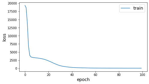
Training
We now create a training generator and fit our model.
[9]:
epochs = 100
[10]:
batch_size = 10
train_gen = generator.flow(batch_size=batch_size, num_parallel_calls=10)

history = model.fit(
    train_gen, epochs=epochs, verbose=1, steps_per_epoch=int(len(G.nodes()) // batch_size)
)
Train for 270 steps
Epoch 1/100
270/270 [==============================] - 1s 5ms/step - loss: 19299.1514
Epoch 2/100
270/270 [==============================] - 1s 4ms/step - loss: 18584.0471
Epoch 3/100
270/270 [==============================] - 1s 4ms/step - loss: 13763.5269
Epoch 4/100
270/270 [==============================] - 1s 4ms/step - loss: 6771.1345
Epoch 5/100
270/270 [==============================] - 1s 4ms/step - loss: 4035.6309
Epoch 6/100
270/270 [==============================] - 1s 4ms/step - loss: 3519.8691
Epoch 7/100
270/270 [==============================] - 1s 3ms/step - loss: 3383.0847
Epoch 8/100
270/270 [==============================] - 1s 3ms/step - loss: 3320.7310
Epoch 9/100
270/270 [==============================] - 1s 3ms/step - loss: 3277.2439
Epoch 10/100
270/270 [==============================] - 1s 3ms/step - loss: 3238.2837
Epoch 11/100
270/270 [==============================] - 1s 3ms/step - loss: 3199.8162
Epoch 12/100
270/270 [==============================] - 1s 3ms/step - loss: 3156.2153
Epoch 13/100
270/270 [==============================] - 1s 4ms/step - loss: 3107.1416
Epoch 14/100
270/270 [==============================] - 1s 3ms/step - loss: 3049.6755
Epoch 15/100
270/270 [==============================] - 1s 3ms/step - loss: 2981.1811
Epoch 16/100
270/270 [==============================] - 1s 3ms/step - loss: 2901.2860
Epoch 17/100
270/270 [==============================] - 1s 3ms/step - loss: 2808.0300
Epoch 18/100
270/270 [==============================] - 1s 3ms/step - loss: 2700.7581
Epoch 19/100
270/270 [==============================] - 1s 3ms/step - loss: 2581.6943
Epoch 20/100
270/270 [==============================] - 1s 3ms/step - loss: 2447.4928
Epoch 21/100
270/270 [==============================] - 1s 4ms/step - loss: 2302.0684
Epoch 22/100
270/270 [==============================] - 1s 4ms/step - loss: 2147.9549
Epoch 23/100
270/270 [==============================] - 1s 4ms/step - loss: 1986.4759
Epoch 24/100
270/270 [==============================] - 1s 4ms/step - loss: 1820.3749
Epoch 25/100
270/270 [==============================] - 1s 4ms/step - loss: 1655.2787
Epoch 26/100
270/270 [==============================] - 1s 4ms/step - loss: 1491.3064
Epoch 27/100
270/270 [==============================] - 1s 4ms/step - loss: 1335.0083
Epoch 28/100
270/270 [==============================] - 1s 4ms/step - loss: 1188.2650
Epoch 29/100
270/270 [==============================] - 1s 4ms/step - loss: 1050.2244
Epoch 30/100
270/270 [==============================] - 1s 4ms/step - loss: 929.6299
Epoch 31/100
270/270 [==============================] - 1s 4ms/step - loss: 822.2163
Epoch 32/100
270/270 [==============================] - 1s 4ms/step - loss: 731.3553
Epoch 33/100
270/270 [==============================] - 1s 4ms/step - loss: 652.2980
Epoch 34/100
270/270 [==============================] - 1s 4ms/step - loss: 586.6967
Epoch 35/100
270/270 [==============================] - 1s 4ms/step - loss: 528.6466
Epoch 36/100
270/270 [==============================] - 1s 4ms/step - loss: 478.4964
Epoch 37/100
270/270 [==============================] - 1s 4ms/step - loss: 434.0944
Epoch 38/100
270/270 [==============================] - 1s 3ms/step - loss: 392.1930
Epoch 39/100
270/270 [==============================] - 1s 4ms/step - loss: 356.2435
Epoch 40/100
270/270 [==============================] - 1s 4ms/step - loss: 324.6430
Epoch 41/100
270/270 [==============================] - 1s 4ms/step - loss: 297.3347
Epoch 42/100
270/270 [==============================] - 1s 4ms/step - loss: 273.8448
Epoch 43/100
270/270 [==============================] - 1s 4ms/step - loss: 253.3782
Epoch 44/100
270/270 [==============================] - 1s 4ms/step - loss: 234.9921
Epoch 45/100
270/270 [==============================] - 1s 4ms/step - loss: 218.5847
Epoch 46/100
270/270 [==============================] - 1s 4ms/step - loss: 203.9068
Epoch 47/100
270/270 [==============================] - 1s 4ms/step - loss: 190.1291
Epoch 48/100
270/270 [==============================] - 1s 4ms/step - loss: 178.2929
Epoch 49/100
270/270 [==============================] - 1s 4ms/step - loss: 167.0052
Epoch 50/100
270/270 [==============================] - 1s 4ms/step - loss: 157.4150
Epoch 51/100
270/270 [==============================] - 1s 4ms/step - loss: 148.5489
Epoch 52/100
270/270 [==============================] - 1s 4ms/step - loss: 140.3815
Epoch 53/100
270/270 [==============================] - 1s 4ms/step - loss: 132.8729
Epoch 54/100
270/270 [==============================] - 1s 4ms/step - loss: 125.9563
Epoch 55/100
270/270 [==============================] - 1s 4ms/step - loss: 119.8609
Epoch 56/100
270/270 [==============================] - 1s 3ms/step - loss: 114.1773
Epoch 57/100
270/270 [==============================] - 1s 4ms/step - loss: 108.9112
Epoch 58/100
270/270 [==============================] - 1s 4ms/step - loss: 104.0912
Epoch 59/100
270/270 [==============================] - 1s 4ms/step - loss: 99.6460
Epoch 60/100
270/270 [==============================] - 1s 4ms/step - loss: 95.5902
Epoch 61/100
270/270 [==============================] - 1s 3ms/step - loss: 91.8379
Epoch 62/100
270/270 [==============================] - 1s 3ms/step - loss: 88.3480
Epoch 63/100
270/270 [==============================] - 1s 4ms/step - loss: 85.1091
Epoch 64/100
270/270 [==============================] - 1s 3ms/step - loss: 82.1819
Epoch 65/100
270/270 [==============================] - 1s 4ms/step - loss: 79.4157
Epoch 66/100
270/270 [==============================] - 1s 4ms/step - loss: 76.8253
Epoch 67/100
270/270 [==============================] - 1s 4ms/step - loss: 74.4604
Epoch 68/100
270/270 [==============================] - 1s 4ms/step - loss: 72.1983
Epoch 69/100
270/270 [==============================] - 1s 3ms/step - loss: 70.1434
Epoch 70/100
270/270 [==============================] - 1s 3ms/step - loss: 68.2032
Epoch 71/100
270/270 [==============================] - 1s 4ms/step - loss: 66.4372
Epoch 72/100
270/270 [==============================] - 1s 4ms/step - loss: 64.7467
Epoch 73/100
270/270 [==============================] - 1s 4ms/step - loss: 63.2199
Epoch 74/100
270/270 [==============================] - 1s 4ms/step - loss: 61.7614
Epoch 75/100
270/270 [==============================] - 1s 4ms/step - loss: 60.4157
Epoch 76/100
270/270 [==============================] - 1s 4ms/step - loss: 59.1597
Epoch 77/100
270/270 [==============================] - 1s 4ms/step - loss: 58.0120
Epoch 78/100
270/270 [==============================] - 1s 4ms/step - loss: 56.8866
Epoch 79/100
270/270 [==============================] - 1s 4ms/step - loss: 55.8909
Epoch 80/100
270/270 [==============================] - 1s 4ms/step - loss: 54.9267
Epoch 81/100
270/270 [==============================] - 1s 4ms/step - loss: 54.0852
Epoch 82/100
270/270 [==============================] - 1s 3ms/step - loss: 53.2545
Epoch 83/100
270/270 [==============================] - 1s 4ms/step - loss: 52.4935
Epoch 84/100
270/270 [==============================] - 1s 4ms/step - loss: 51.8347
Epoch 85/100
270/270 [==============================] - 1s 4ms/step - loss: 51.1775
Epoch 86/100
270/270 [==============================] - 1s 4ms/step - loss: 50.5880
Epoch 87/100
270/270 [==============================] - 1s 4ms/step - loss: 50.0379
Epoch 88/100
270/270 [==============================] - 1s 4ms/step - loss: 49.5201
Epoch 89/100
270/270 [==============================] - 1s 4ms/step - loss: 49.0467
Epoch 90/100
270/270 [==============================] - 1s 4ms/step - loss: 48.6053
Epoch 91/100
270/270 [==============================] - 1s 4ms/step - loss: 48.2098
Epoch 92/100
270/270 [==============================] - 1s 4ms/step - loss: 47.8241
Epoch 93/100
270/270 [==============================] - 1s 4ms/step - loss: 47.4858
Epoch 94/100
270/270 [==============================] - 1s 4ms/step - loss: 47.1706
Epoch 95/100
270/270 [==============================] - 1s 4ms/step - loss: 46.8783
Epoch 96/100
270/270 [==============================] - 1s 3ms/step - loss: 46.6151
Epoch 97/100
270/270 [==============================] - 1s 3ms/step - loss: 46.3614
Epoch 98/100
270/270 [==============================] - 1s 4ms/step - loss: 46.1341
Epoch 99/100
270/270 [==============================] - 1s 3ms/step - loss: 45.9292
Epoch 100/100
270/270 [==============================] - 1s 4ms/step - loss: 45.7389
[11]:
plot_history(history)
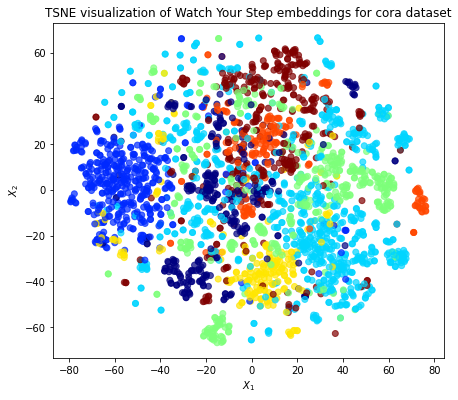
Visualizing Embeddings
Now we use TSNE to visualize the embeddings.
[12]:
embeddings = wys.embeddings()
[13]:
import sklearn
from sklearn.preprocessing import OneHotEncoder
from sklearn.manifold import TSNE

nodelist = list(G.nodes())

labels = subjects.loc[nodelist]
target_encoding = OneHotEncoder(sparse=False)
label_vectors = target_encoding.fit_transform(labels.values.reshape(-1, 1))
[14]:
transform = TSNE

trans = transform(n_components=2)
emb_transformed = pd.DataFrame(trans.fit_transform(embeddings), index=nodelist)

emb_transformed["label"] = np.argmax(label_vectors, 1)
[15]:
alpha = 0.7

fig, ax = plt.subplots(figsize=(7, 7))
ax.scatter(
    emb_transformed[0],
    emb_transformed[1],
    c=emb_transformed["label"].astype("category"),
    cmap="jet",
    alpha=alpha,
)

ax.set(aspect="equal", xlabel="$X_1$", ylabel="$X_2$")
plt.title(
    "{} visualization of Watch Your Step embeddings for cora dataset".format(
        transform.__name__
    )
)
plt.show()
Classification
Here, we predict the class of a node by performing a weighted average of the training labels, with the weights determined by the similarity of that node’s embedding with the training node embeddings.
[16]:
# choose a random set of training nodes by permuting the labels and taking the first 300.
shuffled_idx = np.random.permutation(label_vectors.shape[0])
train_node_idx = shuffled_idx[:300]
test_node_idx = shuffled_idx[300:]

training_labels = label_vectors.copy()
training_labels[test_node_idx] = 0
[17]:
d = embeddings.shape[1] // 2

predictions = np.dot(
    np.exp(np.dot(embeddings[:, :d], embeddings[:, d:].transpose())), training_labels
)

np.mean(
    np.argmax(predictions[test_node_idx], 1) == np.argmax(label_vectors[test_node_idx], 1)
)
[17]:
0.6789867109634552
Execute this notebook:
![]()
![]() Download locally
Download locally
