Execute this notebook:
![]()
![]() Download locally
Download locally
Semi-supervised node classification via GCN, Deep Graph Infomax and fine-tuning
This demo demonstrates how to perform semi-supervised node classification, using the Deep Graph Infomax algorithm and GCN on the Cora dataset. It uses very few labelled training examples, demonstrating the benefits of pre-training a model with Deep Graph Infomax for data scarce environments.
Other related demos:
the GCN node classification demo describes the node classification task in more detail, in a supervised context
the Deep Graph Infomax embeddings demo describes using Deep Graph Infomax in more detail, including applying to algorithms beyond GCN.
This follows the usual StellarGraph workflow:
load the dataset
create our data generators
train our model
We do step 3 three times:
Pre-train a GCN model using Deep Graph Infomax, without any labelled data
Fine-tune that GCN model using the small training set
Train a fresh GCN model from scratch with the training set (no pre-training).
[3]:
import stellargraph as sg
from stellargraph.mapper import CorruptedGenerator, FullBatchNodeGenerator
from stellargraph.layer import GCN, DeepGraphInfomax

import pandas as pd
from sklearn import model_selection, preprocessing
from IPython.display import display, HTML

import tensorflow as tf
from tensorflow.keras import Model, layers, optimizers, callbacks
Loading the graph
(See the “Loading from Pandas” demo for details on how data can be loaded.)
[4]:
dataset = sg.datasets.Cora()
display(HTML(dataset.description))
G, node_classes = dataset.load()
[5]:
print(G.info())
StellarGraph: Undirected multigraph
 Nodes: 2708, Edges: 5429

 Node types:
  paper: [2708]
    Features: float32 vector, length 1433
    Edge types: paper-cites->paper

 Edge types:
    paper-cites->paper: [5429]
        Weights: all 1 (default)
Data Generators
Now we create the data generators using CorruptedGenerator (docs). CorruptedGenerator returns shuffled node features along with the regular node features and we train our model to discriminate between the two.
Note that:
We typically pass all nodes to
corrupted_generator.flowbecause this is an unsupervised taskWe don’t pass
targetstocorrupted_generator.flowbecause these are binary labels (true nodes, false nodes) that are created byCorruptedGenerator
[6]:
fullbatch_generator = FullBatchNodeGenerator(G)

corrupted_generator = CorruptedGenerator(fullbatch_generator)
gen = corrupted_generator.flow(G.nodes())
Using GCN (local pooling) filters...
Model pre-training with Deep Graph Infomax
We create and train our GCN (docs) and DeepGraphInfomax (docs) models. Note that the loss used here must always be tf.nn.sigmoid_cross_entropy_with_logits.
[7]:
def make_gcn_model():
    # function because we want to create a second one with the same parameters later
    return GCN(
        layer_sizes=[16, 16],
        activations=["relu", "relu"],
        generator=fullbatch_generator,
        dropout=0.4,
    )


pretrained_gcn_model = make_gcn_model()
[8]:
infomax = DeepGraphInfomax(pretrained_gcn_model, corrupted_generator)
x_in, x_out = infomax.in_out_tensors()

dgi_model = Model(inputs=x_in, outputs=x_out)
dgi_model.compile(
    loss=tf.nn.sigmoid_cross_entropy_with_logits, optimizer=optimizers.Adam(lr=1e-3)
)
[9]:
epochs = 500
[10]:
dgi_es = callbacks.EarlyStopping(monitor="loss", patience=50, restore_best_weights=True)
dgi_history = dgi_model.fit(gen, epochs=epochs, verbose=0, callbacks=[dgi_es])
[11]:
sg.utils.plot_history(dgi_history)
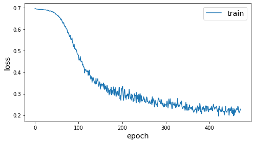
Node classification
We’ve now initialised the weights of the model to capture useful properties of the graph structure and node structure. We can now further train the model to perform a node classification prediction task. To emphasise the value of the unsupervised weights, we will use a very small amount of labelled data for training.
See the GCN node classification demo for more details on this task.
Data preparation
The Cora dataset labels academic papers into one of 7 subjects:
[12]:
node_classes.value_counts().to_frame()
[12]:
| subject | |
|---|---|
| Neural_Networks | 818 |
| Probabilistic_Methods | 426 |
| Genetic_Algorithms | 418 |
| Theory | 351 |
| Case_Based | 298 |
| Reinforcement_Learning | 217 |
| Rule_Learning | 180 |
To simulate a data-poor environment, we will split the data into a train set of size 8, along with test and validation sets.
[13]:
train_classes, test_classes = model_selection.train_test_split(
    node_classes, train_size=8, stratify=node_classes, random_state=1
)
val_classes, test_classes = model_selection.train_test_split(
    test_classes, train_size=500, stratify=test_classes
)
The train set has only one or two observations of each class.
[14]:
train_classes.value_counts().to_frame()
[14]:
| subject | |
|---|---|
| Neural_Networks | 2 |
| Probabilistic_Methods | 1 |
| Rule_Learning | 1 |
| Reinforcement_Learning | 1 |
| Genetic_Algorithms | 1 |
| Theory | 1 |
| Case_Based | 1 |
For a categorical task, the categories need to be one hot encoded.
[15]:
target_encoding = preprocessing.LabelBinarizer()

train_targets = target_encoding.fit_transform(train_classes)
val_targets = target_encoding.transform(val_classes)
test_targets = target_encoding.transform(test_classes)
[16]:
train_gen = fullbatch_generator.flow(train_classes.index, train_targets)
test_gen = fullbatch_generator.flow(test_classes.index, test_targets)
val_gen = fullbatch_generator.flow(val_classes.index, val_targets)
Fine-tuning model
We now have the required pieces to finalise our GCN model for node classification:
a GCN model with weights pre-trained with Deep Graph Infomax to capture the graph structure
a small train set
We use the same GCN model as before but train it for a supervised categorical prediction task. See the fully-supervised GCN node classification demo for more details.
[17]:
pretrained_x_in, pretrained_x_out = pretrained_gcn_model.in_out_tensors()

pretrained_predictions = tf.keras.layers.Dense(
    units=train_targets.shape[1], activation="softmax"
)(pretrained_x_out)
[18]:
pretrained_model = Model(inputs=pretrained_x_in, outputs=pretrained_predictions)
pretrained_model.compile(
    optimizer=optimizers.Adam(lr=0.01), loss="categorical_crossentropy", metrics=["acc"],
)
[19]:
prediction_es = callbacks.EarlyStopping(
    monitor="val_acc", patience=50, restore_best_weights=True
)
[20]:
pretrained_history = pretrained_model.fit(
    train_gen,
    epochs=epochs,
    verbose=0,
    validation_data=val_gen,
    callbacks=[prediction_es],
)
[21]:
sg.utils.plot_history(pretrained_history)
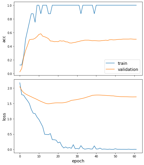
We’ve now fine-tuned our model for node classification. Observe that the accuracy in the first few epochs was very poor, but it quickly improved. (The train accuracy plot is quantised because the training set is so small.)
[22]:
pretrained_test_metrics = dict(
    zip(pretrained_model.metrics_names, pretrained_model.evaluate(test_gen))
)
print(pretrained_test_metrics)
1/1 [==============================] - 0s 920us/step - loss: 1.5896 - acc: 0.5632
{'loss': 1.5896106958389282, 'acc': 0.5631818175315857}
Model without Deep Graph Infomax pre-training
Let’s also train an equivalent GCN model in a fully supervised manner, starting with the same model configuration and using the same 8 training examples.
[23]:
direct_gcn_model = make_gcn_model()
direct_x_in, direct_x_out = direct_gcn_model.in_out_tensors()
direct_predictions = tf.keras.layers.Dense(
    units=train_targets.shape[1], activation="softmax"
)(direct_x_out)
[24]:
direct_model = Model(inputs=direct_x_in, outputs=direct_predictions)
direct_model.compile(
    optimizer=optimizers.Adam(lr=0.01), loss="categorical_crossentropy", metrics=["acc"],
)
[25]:
direct_history = direct_model.fit(
    train_gen,
    epochs=epochs,
    verbose=0,
    validation_data=val_gen,
    callbacks=[prediction_es],
)
[26]:
sg.utils.plot_history(direct_history)
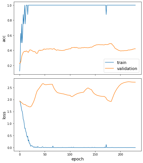
[27]:
direct_test_metrics = dict(
    zip(direct_model.metrics_names, direct_model.evaluate(test_gen))
)
print(direct_test_metrics)
1/1 [==============================] - 0s 946us/step - loss: 2.0196 - acc: 0.4559
{'loss': 2.0196211338043213, 'acc': 0.4559091031551361}
Comparison of model performance
The following table shows the performance of the two models, for comparison.
[28]:
pd.DataFrame(
    [pretrained_test_metrics, direct_test_metrics],
    index=["with DGI pre-training", "without pre-training"],
).round(3)
[28]:
| loss | acc | |
|---|---|---|
| with DGI pre-training | 1.59 | 0.563 |
| without pre-training | 2.02 | 0.456 |
Conclusion
In this demo, we performed semi-supervised node classification on the Cora dataset. This example had extreme data scarcity: only 8 labelled training examples, with one or two from each of the 7 classes. We used Deep Graph Infomax to train a GCN model on the whole Cora graph, without labels. We then further trained this GCN model in the normal manner, to fine-tuned its weights on the small set of labelled data. The GCN model pre-trained with Deep Graph Infomax outperforms a GCN model without any such pre-training.
Execute this notebook:
![]()
![]() Download locally
Download locally
