Execute this notebook: Download locally

Cluster GCN on Neo4j

This example demonstrates how to run Cluster GCN on a dataset stored entirely on disk with Neo4j. Our Neo4j Cluster GCN implementation iterates through user specified graph clusters and only ever stores the edges and features of one cluster in memory at any given time. This enables Cluster GCN to be used on extremely large datasets that don’t fit into memory.

We use Cora here as an example, see this notebook for instructions on how to load the Cora dataset into Neo4j.

import stellargraph as sg
from stellargraph.connector.neo4j import Neo4jStellarGraph
from stellargraph.layer import ClusterGCN
from stellargraph.mapper import ClusterNodeGenerator
import tensorflow as tf
import py2neo
import os
from sklearn import preprocessing, feature_extraction, model_selection

import numpy as np
import scipy.sparse as sps
import pandas as pd

Connect to Neo4j

First we connect to the Neo4j with py2neo, we then create a Neo4jStellarGraph object.

default_host = os.environ.get("STELLARGRAPH_NEO4J_HOST")

# Create the Neo4j Graph database object;
# the arguments can be edited to specify location and authentication
graph = py2neo.Graph(host=default_host, port=None, user=None, password="pass")
neo4j_sg = Neo4jStellarGraph(graph)

Data labels

Here we get the node labels. Cluster GCN is semi-supervised and requires labels to be specified for some nodes.

# read the node labels from a seperate file
# note this function also returns a StellarGraph
# which we won't be using for this demo - we only need Neo4jStellarGraph!
_, labels = sg.datasets.Cora().load()

# split the node labels into train/test/val

train_labels, test_labels = model_selection.train_test_split(
    labels, train_size=140, test_size=None, stratify=labels
)
val_labels, test_labels = model_selection.train_test_split(
    test_labels, train_size=500, test_size=None, stratify=test_labels
)

target_encoding = preprocessing.LabelBinarizer()

train_targets = target_encoding.fit_transform(train_labels)
val_targets = target_encoding.transform(val_labels)
test_targets = target_encoding.transform(test_labels)

Neo4j Clustering

We use one of the Neo4j Data Science Library’s community detection algorithms to split our graph into clusters for ClusterGCN.

We can use:

• “louvain”: https://neo4j.com/docs/graph-data-science/current/algorithms/louvain/

• “labelPropagation”: https://neo4j.com/docs/graph-data-science/current/algorithms/label-propagation/=

clusters = neo4j_sg.clusters(method="louvain")

Keras sequences

We now use StellarGraph to create keras sequences for taining, testing, and validation. Under the hood, these sequences connect to your Neo4j database and lazily load data for each cluster.

# create the Neo4jClusterNodeGenerator
# and the keras sequence objects

generator = ClusterNodeGenerator(neo4j_sg, clusters=clusters)

train_gen = generator.flow(train_labels.index, targets=train_targets)
val_gen = generator.flow(val_labels.index, targets=val_targets)
test_gen = generator.flow(test_labels.index, targets=test_targets)

Number of clusters 173
0 cluster has size 118
1 cluster has size 413
2 cluster has size 167
3 cluster has size 38
4 cluster has size 67
5 cluster has size 226
6 cluster has size 18
7 cluster has size 68
8 cluster has size 26
9 cluster has size 60
10 cluster has size 83
11 cluster has size 118
12 cluster has size 73
13 cluster has size 3
14 cluster has size 22
15 cluster has size 36
16 cluster has size 237
17 cluster has size 12
18 cluster has size 1
19 cluster has size 128
20 cluster has size 41
21 cluster has size 11
22 cluster has size 60
23 cluster has size 5
24 cluster has size 3
25 cluster has size 100
26 cluster has size 27
27 cluster has size 1
28 cluster has size 39
29 cluster has size 2
30 cluster has size 18
31 cluster has size 11
32 cluster has size 3
33 cluster has size 5
34 cluster has size 8
35 cluster has size 14
36 cluster has size 3
37 cluster has size 2
38 cluster has size 51
39 cluster has size 2
40 cluster has size 5
41 cluster has size 4
42 cluster has size 10
43 cluster has size 5
44 cluster has size 15
45 cluster has size 5
46 cluster has size 1
47 cluster has size 4
48 cluster has size 3
49 cluster has size 6
50 cluster has size 1
51 cluster has size 3
52 cluster has size 6
53 cluster has size 8
54 cluster has size 2
55 cluster has size 2
56 cluster has size 1
57 cluster has size 13
58 cluster has size 1
59 cluster has size 6
60 cluster has size 1
61 cluster has size 10
62 cluster has size 10
63 cluster has size 5
64 cluster has size 2
65 cluster has size 4
66 cluster has size 12
67 cluster has size 3
68 cluster has size 2
69 cluster has size 5
70 cluster has size 1
71 cluster has size 2
72 cluster has size 1
73 cluster has size 2
74 cluster has size 2
75 cluster has size 2
76 cluster has size 2
77 cluster has size 1
78 cluster has size 2
79 cluster has size 2
80 cluster has size 9
81 cluster has size 1
82 cluster has size 2
83 cluster has size 2
84 cluster has size 1
85 cluster has size 2
86 cluster has size 2
87 cluster has size 2
88 cluster has size 1
89 cluster has size 1
90 cluster has size 2
91 cluster has size 2
92 cluster has size 1
93 cluster has size 1
94 cluster has size 2
95 cluster has size 1
96 cluster has size 2
97 cluster has size 2
98 cluster has size 2
99 cluster has size 2
100 cluster has size 3
101 cluster has size 5
102 cluster has size 5
103 cluster has size 4
104 cluster has size 1
105 cluster has size 13
106 cluster has size 1
107 cluster has size 3
108 cluster has size 3
109 cluster has size 2
110 cluster has size 2
111 cluster has size 3
112 cluster has size 2
113 cluster has size 1
114 cluster has size 1
115 cluster has size 1
116 cluster has size 2
117 cluster has size 3
118 cluster has size 2
119 cluster has size 2
120 cluster has size 2
121 cluster has size 2
122 cluster has size 12
123 cluster has size 1
124 cluster has size 4
125 cluster has size 1
126 cluster has size 2
127 cluster has size 2
128 cluster has size 1
129 cluster has size 2
130 cluster has size 1
131 cluster has size 2
132 cluster has size 8
133 cluster has size 2
134 cluster has size 2
135 cluster has size 2
136 cluster has size 1
137 cluster has size 2
138 cluster has size 1
139 cluster has size 2
140 cluster has size 3
141 cluster has size 1
142 cluster has size 2
143 cluster has size 4
144 cluster has size 2
145 cluster has size 2
146 cluster has size 2
147 cluster has size 2
148 cluster has size 2
149 cluster has size 2
150 cluster has size 2
151 cluster has size 2
152 cluster has size 1
153 cluster has size 4
154 cluster has size 1
155 cluster has size 3
156 cluster has size 2
157 cluster has size 2
158 cluster has size 1
159 cluster has size 1
160 cluster has size 3
161 cluster has size 2
162 cluster has size 1
163 cluster has size 2
164 cluster has size 2
165 cluster has size 2
166 cluster has size 2
167 cluster has size 1
168 cluster has size 2
169 cluster has size 2
170 cluster has size 1
171 cluster has size 2
172 cluster has size 2

Create and train your model!

Now we create and train the Cluster GCN model.

# create the model
cluster_gcn = ClusterGCN(
    layer_sizes=[32, 32], generator=generator, activations=["relu", "relu"], dropout=0.5,
)

x_in, x_out = cluster_gcn.in_out_tensors()
predictions = tf.keras.layers.Dense(units=val_targets.shape[1], activation="softmax")(
    x_out
)
model = tf.keras.Model(x_in, predictions)
model.compile(
    optimizer=tf.keras.optimizers.Adam(lr=0.01),
    loss=tf.keras.losses.categorical_crossentropy,
    metrics=["acc"],
)

# train the model!
history = model.fit(train_gen, validation_data=val_gen, epochs=10)

  ['...']
  ['...']
Train for 173 steps, validate for 173 steps
Epoch 1/10
173/173 [==============================] - 9s 50ms/step - loss: 0.4474 - acc: 0.2357 - val_loss: 0.8697 - val_acc: 0.3040
Epoch 2/10
173/173 [==============================] - 7s 41ms/step - loss: 0.3968 - acc: 0.3786 - val_loss: 0.6322 - val_acc: 0.6740
Epoch 3/10
173/173 [==============================] - 7s 42ms/step - loss: 0.2307 - acc: 0.5500 - val_loss: 0.7893 - val_acc: 0.4980
Epoch 4/10
173/173 [==============================] - 7s 41ms/step - loss: 0.1732 - acc: 0.6214 - val_loss: 0.7399 - val_acc: 0.5860
Epoch 5/10
173/173 [==============================] - 7s 42ms/step - loss: 0.1245 - acc: 0.8000 - val_loss: 0.8939 - val_acc: 0.6680
Epoch 6/10
173/173 [==============================] - 7s 41ms/step - loss: 0.1719 - acc: 0.8500 - val_loss: 1.3818 - val_acc: 0.5820
Epoch 7/10
173/173 [==============================] - 7s 41ms/step - loss: 0.1494 - acc: 0.8357 - val_loss: 0.9496 - val_acc: 0.7220
Epoch 8/10
173/173 [==============================] - 7s 41ms/step - loss: 0.1257 - acc: 0.8929 - val_loss: 0.7883 - val_acc: 0.7200
Epoch 9/10
173/173 [==============================] - 7s 40ms/step - loss: 0.1114 - acc: 0.9286 - val_loss: 0.6892 - val_acc: 0.7140
Epoch 10/10
173/173 [==============================] - 7s 42ms/step - loss: 0.1298 - acc: 0.8929 - val_loss: 0.7618 - val_acc: 0.7320

# evaluate the model
model.evaluate(test_gen)

  ['...']
173/173 [==============================] - 4s 21ms/step - loss: 1.4353 - acc: 0.7689

[1.4352797645499302, 0.7688588]

sg.utils.plot_history(history)

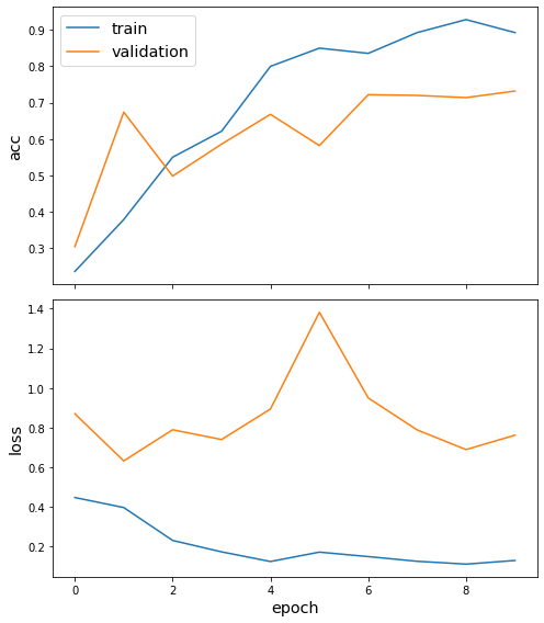
And that’s it! We’ve trained a graph neural network without ever loading the whole graph into memory.

Please refer to cluster-gcn-node-classification for node embedding visualization.

Execute this notebook: Download locally