Cluster-GCN for node classification
Run the master version of this notebook: |
This notebook demonstrates how to use StellarGraph’s implementation of Cluster-GCN, [1], for node classification on a homogeneous graph.
Cluster-GCN is an extension of the Graph Convolutional Network (GCN) algorithm, [2], for scalable training of deeper Graph Neural Networks using Stochastic Gradient Descent (SGD).
As a first step, Cluster-GCN splits a given graph into k non-overlapping subgraphs, i.e., no two subgraphs share a node. In [1], it is suggested that for best classification performance, the METIS graph clustering algorithm, [3], should be utilised; METIS groups together nodes that form a well connected neighborhood with few connections to other subgraphs. The default clustering algorithm StellarGraph uses is the random assignment of nodes to clusters. The user is free to use any
suitable clustering algorithm to determine the clusters before training the Cluster-GCN model.
This notebook demonstrates how to use either random clustering or METIS. For the latter, it is necessary that 3rd party software has correctly been installed; later, we provide links to websites that host the software and provide detailed installation instructions.
During model training, each subgraph or combination of subgraphs is treated as a mini-batch for estimating the parameters of a GCN model. A pass over all subgraphs is considered a training epoch.
Cluster-GCN further extends GCN from the transductive to the inductive setting but this is not demonstrated in this notebook.
This notebook demonstrates Cluster-GCN for node classification using 2 citation network datasets, Cora and PubMed-Diabetes.
References
[1] Cluster-GCN: An Efficient Algorithm for Training Deep and Large Graph Convolutional Networks. W. Chiang, X. Liu, S. Si, Y. Li, S. Bengio, and C. Hsiej, KDD, 2019, arXiv:1905.07953 (download link)
[2] Semi-Supervised Classification with Graph Convolutional Networks. T. Kipf, M. Welling. ICLR 2017. arXiv:1609.02907 (download link)
[3] METIS: Serial Graph Partitioning and Fill-reducing Matrix Ordering. (download link)
[1]:
# install StellarGraph if running on Google Colab
import sys
if 'google.colab' in sys.modules:
  %pip install -q stellargraph[demos]==1.0.0rc1
[2]:
# verify that we're using the correct version of StellarGraph for this notebook
import stellargraph as sg

try:
    sg.utils.validate_notebook_version("1.0.0rc1")
except AttributeError:
    raise ValueError(
        f"This notebook requires StellarGraph version 1.0.0rc1, but a different version {sg.__version__} is installed.  Please see <https://github.com/stellargraph/stellargraph/issues/1172>."
    ) from None
[3]:
import networkx as nx
import pandas as pd
import itertools
import json
import os

import numpy as np

from networkx.readwrite import json_graph

from sklearn.preprocessing import StandardScaler

import stellargraph as sg
from stellargraph.mapper import ClusterNodeGenerator
from stellargraph.layer import ClusterGCN
from stellargraph import globalvar

from tensorflow.keras import backend as K

from tensorflow.keras import layers, optimizers, losses, metrics, Model
from sklearn import preprocessing, feature_extraction, model_selection
from stellargraph import datasets
from IPython.display import display, HTML
from IPython.display import display, HTML
import matplotlib.pyplot as plt
%matplotlib inline
Loading the dataset
This notebook demonstrates node classification using the Cluster-GCN algorithm using one of two citation networks, Cora and Pubmed.
[4]:
display(HTML(datasets.Cora().description))
display(HTML(datasets.PubMedDiabetes().description))
[5]:
dataset = "cora"  # can also select 'pubmed'

if dataset == "cora":
    G, labels = datasets.Cora().load()
elif dataset == "pubmed":
    G, labels = datasets.PubMedDiabetes().load()
[6]:
print(G.info())
StellarGraph: Undirected multigraph
 Nodes: 2708, Edges: 5429

 Node types:
  paper: [2708]
    Features: float32 vector, length 1433
    Edge types: paper-cites->paper

 Edge types:
    paper-cites->paper: [5429]
[7]:
set(labels)
[7]:
{'Case_Based',
 'Genetic_Algorithms',
 'Neural_Networks',
 'Probabilistic_Methods',
 'Reinforcement_Learning',
 'Rule_Learning',
 'Theory'}
Splitting the data
We aim to train a graph-ML model that will predict the subject or label (depending on the dataset) attribute on the nodes.
For machine learning we want to take a subset of the nodes for training, and use the rest for validation and testing. We’ll use scikit-learn again to do this.
The number of labeled nodes we use for training depends on the dataset. We use 140 labeled nodes for Cora and 60 for Pubmed training. The validation and test sets have the same sizes for both datasets. We use 500 nodes for validation and the rest for testing.
[8]:
if dataset == "cora":
    train_size = 140
elif dataset == "pubmed":
    train_size = 60

train_labels, test_labels = model_selection.train_test_split(
    labels, train_size=train_size, test_size=None, stratify=labels
)
val_labels, test_labels = model_selection.train_test_split(
    test_labels, train_size=500, test_size=None, stratify=test_labels
)
Note using stratified sampling gives the following counts:
[9]:
from collections import Counter

Counter(train_labels)
[9]:
Counter({'Neural_Networks': 42,
         'Probabilistic_Methods': 22,
         'Reinforcement_Learning': 11,
         'Genetic_Algorithms': 22,
         'Case_Based': 16,
         'Theory': 18,
         'Rule_Learning': 9})
The training set has class imbalance that might need to be compensated, e.g., via using a weighted cross-entropy loss in model training, with class weights inversely proportional to class support. However, we will ignore the class imbalance in this example, for simplicity.
Converting to numeric arrays
For our categorical target, we will use one-hot vectors that will be fed into a soft-max Keras layer during training.
[10]:
target_encoding = preprocessing.LabelBinarizer()

train_targets = target_encoding.fit_transform(train_labels)
val_targets = target_encoding.transform(val_labels)
test_targets = target_encoding.transform(test_labels)
Next, we prepare a Pandas DataFrame holding the node attributes we want to use to predict the subject. These are the feature vectors that the Keras model will use as input. Cora contains attributes ‘w_x’ that correspond to words found in that publication. If a word occurs more than once in a publication the relevant attribute will be set to one, otherwise it will be zero. Pubmed has similar feature vectors associated with each node but the values are
tf-idf.
Train using cluster GCN
Graph Clustering
Cluster-GCN requires that a graph is clustered into k non-overlapping subgraphs. These subgraphs are used as batches to train a GCN model.
Any graph clustering method can be used, including random clustering that is the default clustering method in StellarGraph.
However, the choice of clustering algorithm can have a large impact on performance. In the Cluster-GCN paper, [1], it is suggested that the METIS algorithm is used as it produces subgraphs that are well connected with few intra-graph edges.
This demo uses random clustering by default.
In order to use METIS, you must download and install the official implemention from here. Also, you must install the Python metis library by following the instructions here.
[11]:
number_of_clusters = 10  # the number of clusters/subgraphs
clusters_per_batch = 2  # combine two cluster per batch
random_clusters = True  # Set to False if you want to use METIS for clustering
[12]:
node_ids = np.array(G.nodes())
[13]:
if random_clusters:
    # We don't have to specify the cluster because the CluserNodeGenerator will take
    # care of the random clustering for us.
    clusters = number_of_clusters
else:
    # We are going to use the METIS clustering algorith,
    print("Graph clustering using the METIS algorithm.")

    import metis

    lil_adj = G.to_adjacency_matrix().tolil()
    adjlist = [tuple(neighbours) for neighbours in lil_adj.rows]

    edgecuts, parts = metis.part_graph(adjlist, number_of_clusters)
    parts = np.array(parts)
    clusters = []
    cluster_ids = np.unique(parts)
    for cluster_id in cluster_ids:
        mask = np.where(parts == cluster_id)
        clusters.append(node_ids[mask])
Next we create the ClusterNodeGenerator object that will give us access to a generator suitable for model training, evaluation, and prediction via the Keras API.
We specify the number of clusters and the number of clusters to combine per batch, q.
[14]:
generator = ClusterNodeGenerator(G, clusters=clusters, q=clusters_per_batch, lam=0.1)
Number of clusters 10
0 cluster has size 270
1 cluster has size 270
2 cluster has size 270
3 cluster has size 270
4 cluster has size 270
5 cluster has size 270
6 cluster has size 270
7 cluster has size 270
8 cluster has size 270
9 cluster has size 278
Now we can specify our machine learning model, we need a few more parameters for this:
- the
layer_sizesis a list of hidden feature sizes of each layer in the model. In this example we use two GCN layers with 32-dimensional hidden node features at each layer. activationsis a list of activations applied to each layer’s outputdropout=0.5specifies a 50% dropout at each layer.
We create the Cluster-GCN model as follows:
[15]:
cluster_gcn = ClusterGCN(
    layer_sizes=[32, 32], activations=["relu", "relu"], generator=generator, dropout=0.5
)
To create a Keras model we now expose the input and output tensors of the Cluster-GCN model for node prediction, via the ClusterGCN.in_out_tensors method:
[16]:
x_inp, x_out = cluster_gcn.in_out_tensors()
[17]:
x_inp
[17]:
[<tf.Tensor 'input_1:0' shape=(1, None, 1433) dtype=float32>,
 <tf.Tensor 'input_2:0' shape=(1, None) dtype=int32>,
 <tf.Tensor 'input_3:0' shape=(1, None, None) dtype=float32>]
[18]:
x_out
[18]:
<tf.Tensor 'gather_indices/Identity:0' shape=(1, None, 32) dtype=float32>
We are also going to add a final layer dense layer with softmax output activation. This layers performs classification so we set the number of units to equal the number of classes.
[19]:
predictions = layers.Dense(units=train_targets.shape[1], activation="softmax")(x_out)
[20]:
predictions
[20]:
<tf.Tensor 'dense/Identity:0' shape=(1, None, 7) dtype=float32>
Finally, we build the Tensorflow model and compile it specifying the loss function, optimiser, and metrics to monitor.
[21]:
model = Model(inputs=x_inp, outputs=predictions)
model.compile(
    optimizer=optimizers.Adam(lr=0.01),
    loss=losses.categorical_crossentropy,
    metrics=["acc"],
)
Train the model
We are now ready to train the ClusterGCN model, keeping track of its loss and accuracy on the training set, and its generalisation performance on a validation set.
We need two generators, one for training and one for validation data. We can create such generators by calling the flow method of the ClusterNodeGenerator object we created earlier and specifying the node IDs and corresponding ground truth target values for each of the two datasets.
[22]:
train_gen = generator.flow(train_labels.index, train_targets, name="train")
val_gen = generator.flow(val_labels.index, val_targets, name="val")
Finally, we are ready to train our ClusterGCN model by calling the fit method of our Tensorflow Keras model.
[23]:
history = model.fit(
    train_gen, validation_data=val_gen, epochs=20, verbose=1, shuffle=False
)
  ['...']
  ['...']
Train for 5 steps, validate for 5 steps
Epoch 1/20
5/5 [==============================] - 1s 147ms/step - loss: 1.8824 - acc: 0.2214 - val_loss: 1.7955 - val_acc: 0.3040
Epoch 2/20
5/5 [==============================] - 0s 22ms/step - loss: 1.6687 - acc: 0.2929 - val_loss: 1.6810 - val_acc: 0.3020
Epoch 3/20
5/5 [==============================] - 0s 21ms/step - loss: 1.5002 - acc: 0.3429 - val_loss: 1.5643 - val_acc: 0.3900
Epoch 4/20
5/5 [==============================] - 0s 21ms/step - loss: 1.2585 - acc: 0.5357 - val_loss: 1.4264 - val_acc: 0.5500
Epoch 5/20
5/5 [==============================] - 0s 21ms/step - loss: 0.9910 - acc: 0.7071 - val_loss: 1.2739 - val_acc: 0.5880
Epoch 6/20
5/5 [==============================] - 0s 22ms/step - loss: 0.8021 - acc: 0.6857 - val_loss: 1.1933 - val_acc: 0.6080
Epoch 7/20
5/5 [==============================] - 0s 21ms/step - loss: 0.6358 - acc: 0.7786 - val_loss: 1.0825 - val_acc: 0.6420
Epoch 8/20
5/5 [==============================] - 0s 21ms/step - loss: 0.5681 - acc: 0.8357 - val_loss: 1.0657 - val_acc: 0.6380
Epoch 9/20
5/5 [==============================] - 0s 22ms/step - loss: 0.4167 - acc: 0.8571 - val_loss: 1.1342 - val_acc: 0.6360
Epoch 10/20
5/5 [==============================] - 0s 21ms/step - loss: 0.3251 - acc: 0.9071 - val_loss: 1.2399 - val_acc: 0.6320
Epoch 11/20
5/5 [==============================] - 0s 21ms/step - loss: 0.2713 - acc: 0.9071 - val_loss: 1.1463 - val_acc: 0.6500
Epoch 12/20
5/5 [==============================] - 0s 21ms/step - loss: 0.3365 - acc: 0.8857 - val_loss: 1.1205 - val_acc: 0.6500
Epoch 13/20
5/5 [==============================] - 0s 22ms/step - loss: 0.2272 - acc: 0.9071 - val_loss: 1.1753 - val_acc: 0.6560
Epoch 14/20
5/5 [==============================] - 0s 21ms/step - loss: 0.2948 - acc: 0.9000 - val_loss: 1.2997 - val_acc: 0.6340
Epoch 15/20
5/5 [==============================] - 0s 21ms/step - loss: 0.2840 - acc: 0.9000 - val_loss: 1.3871 - val_acc: 0.6200
Epoch 16/20
5/5 [==============================] - 0s 22ms/step - loss: 0.1464 - acc: 0.9357 - val_loss: 1.4344 - val_acc: 0.6220
Epoch 17/20
5/5 [==============================] - 0s 22ms/step - loss: 0.2943 - acc: 0.9214 - val_loss: 1.3791 - val_acc: 0.6200
Epoch 18/20
5/5 [==============================] - 0s 21ms/step - loss: 0.1368 - acc: 0.9714 - val_loss: 1.3297 - val_acc: 0.6260
Epoch 19/20
5/5 [==============================] - 0s 21ms/step - loss: 0.1462 - acc: 0.9500 - val_loss: 1.3450 - val_acc: 0.6360
Epoch 20/20
5/5 [==============================] - 0s 23ms/step - loss: 0.1845 - acc: 0.9429 - val_loss: 1.3614 - val_acc: 0.6380
Plot the training history:
[24]:
sg.utils.plot_history(history)
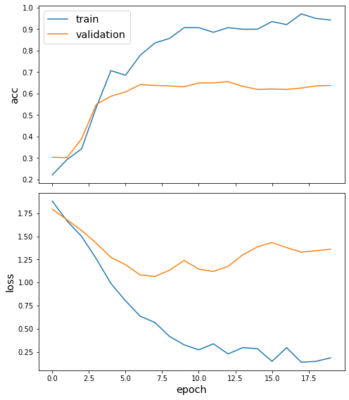
Evaluate the best model on the test set.
Note that Cluster-GCN performance can be very poor if using random graph clustering. Using METIS instead of random graph clustering produces considerably better results.
[25]:
test_gen = generator.flow(test_labels.index, test_targets)
[26]:
test_metrics = model.evaluate(test_gen)
print("\nTest Set Metrics:")
for name, val in zip(model.metrics_names, test_metrics):
    print("\t{}: {:0.4f}".format(name, val))
  ['...']
5/5 [==============================] - 0s 7ms/step - loss: 1.4908 - acc: 0.6291

Test Set Metrics:
        loss: 1.4908
        acc: 0.6291
Making predictions with the model
For predictions to work correctly, we need to remove the extra batch dimensions necessary for the implementation of Cluster-GCN to work. We can easily achieve this by adding a layer after the dense predictions layer to remove this extra dimension.
[27]:
predictions_flat = layers.Lambda(lambda x: K.squeeze(x, 0))(predictions)
[28]:
# Notice that we have removed the first dimension
predictions, predictions_flat
[28]:
(<tf.Tensor 'dense/Identity:0' shape=(1, None, 7) dtype=float32>,
 <tf.Tensor 'lambda/Identity:0' shape=(None, 7) dtype=float32>)
Now let’s get the predictions for all nodes.
We need to create a new model using the same as before input Tensor and our new predictions_flat Tensor as the output. We are going to re-use the trained model weights.
[29]:
model_predict = Model(inputs=x_inp, outputs=predictions_flat)
[30]:
all_nodes = list(G.nodes())
all_gen = generator.flow(all_nodes, name="all_gen")
all_predictions = model_predict.predict(all_gen)
[31]:
all_predictions.shape
[31]:
(2708, 7)
These predictions will be the output of the softmax layer, so to get final categories we’ll use the inverse_transform method of our target attribute specifcation to turn these values back to the original categories.
[32]:
node_predictions = target_encoding.inverse_transform(all_predictions)
Let’s have a look at a few predictions after training the model:
[33]:
len(all_gen.node_order)
[33]:
2708
[34]:
results = pd.Series(node_predictions, index=all_gen.node_order)
df = pd.DataFrame({"Predicted": results, "True": labels})
df.head(10)
[34]:
| Predicted | True | |
|---|---|---|
| 35 | Genetic_Algorithms | Genetic_Algorithms |
| 40 | Genetic_Algorithms | Genetic_Algorithms |
| 114 | Reinforcement_Learning | Reinforcement_Learning |
| 117 | Reinforcement_Learning | Reinforcement_Learning |
| 128 | Reinforcement_Learning | Reinforcement_Learning |
| 130 | Probabilistic_Methods | Reinforcement_Learning |
| 164 | Theory | Theory |
| 288 | Genetic_Algorithms | Reinforcement_Learning |
| 424 | Case_Based | Rule_Learning |
| 434 | Case_Based | Reinforcement_Learning |
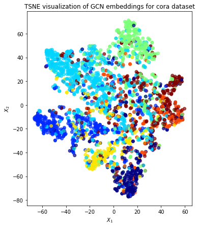
Node embeddings
Evaluate node embeddings as activations of the output of the last graph convolution layer in the ClusterGCN layer stack and visualise them, coloring nodes by their true subject label. We expect to see nice clusters of papers in the node embedding space, with papers of the same subject belonging to the same cluster.
To calculate the node embeddings rather than the class predictions, we create a new model with the same inputs as we used previously x_inp but now the output is the embeddings x_out rather than the predicted class. Additionally note that the weights trained previously are kept in the new model.
Note that the embeddings from the ClusterGCN model have a batch dimension of 1 so we squeeze this to get a matrix of \(N_{nodes} \times N_{emb}\).
[35]:
x_out_flat = layers.Lambda(lambda x: K.squeeze(x, 0))(x_out)
embedding_model = Model(inputs=x_inp, outputs=x_out_flat)
[36]:
emb = embedding_model.predict(all_gen, verbose=1)
emb.shape
5/5 [==============================] - 0s 14ms/step
[36]:
(2708, 32)
Project the embeddings to 2d using either TSNE or PCA transform, and visualise, coloring nodes by their true subject label
[37]:
from sklearn.decomposition import PCA
from sklearn.manifold import TSNE
import pandas as pd
import numpy as np
Prediction Node Order
The predictions are not returned in the same order as the input nodes given. The generator object internally maintains the order of predictions. These are stored in the object’s member variable node_order. We use node_order to re-index the node_data DataFrame such that the prediction order in y corresponds to that of node embeddings in X.
[38]:
X = emb
y = np.argmax(
    target_encoding.transform(labels.reindex(index=all_gen.node_order)), axis=1,
)
[39]:
if X.shape[1] > 2:
    transform = TSNE  # or use PCA for speed

    trans = transform(n_components=2)
    emb_transformed = pd.DataFrame(trans.fit_transform(X), index=all_gen.node_order)
    emb_transformed["label"] = y
else:
    emb_transformed = pd.DataFrame(X, index=list(G.nodes()))
    emb_transformed = emb_transformed.rename(columns={"0": 0, "1": 1})
    emb_transformed["label"] = y
[40]:
alpha = 0.7

fig, ax = plt.subplots(figsize=(7, 7))
ax.scatter(
    emb_transformed[0],
    emb_transformed[1],
    c=emb_transformed["label"].astype("category"),
    cmap="jet",
    alpha=alpha,
)
ax.set(aspect="equal", xlabel="$X_1$", ylabel="$X_2$")
plt.title(
    "{} visualization of GCN embeddings for cora dataset".format(transform.__name__)
)
plt.show()
Run the master version of this notebook: |