Node Representation Learning with attri2vec on Citeseer
Run the master version of this notebook: |
This is the python implementation of the attri2vec algorithm outlined in paper *`Attributed Network Embedding Via Subspace Discovery <https://arxiv.org/abs/1901.04095>`__* D. Zhang, Y. Jie, X. Zhu and C. Zhang, arXiv:1901.04095, [cs.SI], 2019. The implementation uses the stellargraph libraries.
attri2vec
attri2vec learns node representations by performing a linear/non-linear mapping on node content attributes. To make the learned node representations respect structural similarity, `DeepWalk <https://dl.acm.org/citation.cfm?id=2623732>`__/`node2vec <https://snap.stanford.edu/node2vec>`__ learning mechanism is used to make nodes sharing similar random walk context nodes represented closely in the subspace, which is achieved by maximizing the occurrence probability of context nodes
conditioned on the representation of the target nodes. The probability is modelled by Softmax and negative sampling is used to speed up its calculation. This makes attri2vec equivalent to predict whether a node occurs in the given target node’s context in random walks with the representation of the target node, by minimizing the cross-entropy loss.
In implementation, node embeddings are learnt by solving a simple classification task: given a large set of “positive” (target, context) node pairs generated from random walks performed on the graph (i.e., node pairs that co-occur within a certain context window in random walks), and an equally large set of “negative” node pairs that are randomly selected from the graph according to a certain distribution, learn a binary classifier that predicts whether arbitrary node pairs are likely to
co-occur in a random walk performed on the graph. Through learning this simple binary node-pair-classification task, the model automatically learns an inductive mapping from attributes of nodes to node embeddings in a low-dimensional vector space, which preserves structural and feature similarities of the nodes.
To train the attri2vec model, we first construct a training set of nodes, which is composed of an equal number of positive and negative (target, context) pairs from the graph. The positive (target, context) pairs are the node pairs co-occurring on random walks over the graph whereas the negative node pairs are the sampled randomly from the global node degree distribution of the graph. In attri2vec, each node is attached with two kinds of embeddings: 1) the inductive ‘input embedding’,
i.e, the objective embedding, obtained by perform a linear/non-linear transformation on node content features, and 2) ‘output embedding’, i.e., the parameter vector used to predict its occurrence as a context node, obtained by looking up a parameter table. Given a (target, context) pair, attri2vec outputs a predictive value to indicate whether it is positive or negative, which is obtained by performing the dot product of the ‘input embedding’ of the target node and the ‘output embedding’ of
the context node, followed by a sigmoid activation.
The entire model is trained end-to-end by minimizing the binary cross-entropy loss function with regards to predicted node pair labels and true node pair labels, using stochastic gradient descent (SGD) updates of the model parameters, with minibatches of ‘training’ node pairs generated on demand and fed into the model.
[1]:
# install StellarGraph if running on Google Colab
import sys
if 'google.colab' in sys.modules:
  %pip install -q stellargraph[demos]==1.0.0rc1
[2]:
# verify that we're using the correct version of StellarGraph for this notebook
import stellargraph as sg

try:
    sg.utils.validate_notebook_version("1.0.0rc1")
except AttributeError:
    raise ValueError(
        f"This notebook requires StellarGraph version 1.0.0rc1, but a different version {sg.__version__} is installed.  Please see <https://github.com/stellargraph/stellargraph/issues/1172>."
    ) from None
[3]:
import networkx as nx
import pandas as pd
import numpy as np
import os
import random

import stellargraph as sg
from stellargraph.data import UnsupervisedSampler
from stellargraph.mapper import Attri2VecLinkGenerator, Attri2VecNodeGenerator
from stellargraph.layer import Attri2Vec, link_classification

from tensorflow import keras

from pandas.core.indexes.base import Index

import matplotlib.pyplot as plt
from sklearn.manifold import TSNE
from sklearn.decomposition import PCA

from sklearn.model_selection import train_test_split
from sklearn.linear_model import LogisticRegressionCV
from sklearn.metrics import accuracy_score
from stellargraph import datasets
from IPython.display import display, HTML
Dataset
For clarity we ignore isolated nodes and subgraphs and use only the largest connected component.
[4]:
dataset = datasets.CiteSeer()
display(HTML(dataset.description))
G, subjects = dataset.load(largest_connected_component_only=True)
[5]:
print(G.info())
StellarGraph: Undirected multigraph
 Nodes: 2110, Edges: 3757

 Node types:
  paper: [2110]
    Features: float32 vector, length 3703
    Edge types: paper-cites->paper

 Edge types:
    paper-cites->paper: [3757]
Train attri2vec on Citeseer
Specify the other optional parameter values: root nodes, the number of walks to take per node, the length of each walk.
[6]:
nodes = list(G.nodes())
number_of_walks = 4
length = 5
Create the UnsupervisedSampler instance with the relevant parameters passed to it.
[7]:
unsupervised_samples = UnsupervisedSampler(
    G, nodes=nodes, length=length, number_of_walks=number_of_walks
)
Set the batch size and the number of epochs.
[8]:
batch_size = 50
epochs = 4
Define an attri2vec generator, which generates batches of (target, context) nodes and labels for the node pair.
[9]:
generator = Attri2VecLinkGenerator(G, batch_size)
Building the model: a 1-hidden-layer node representation (‘input embedding’) of the target node and the parameter vector (‘output embedding’) for predicting the existence of context node for each (target context) pair, with a link classification layer performed on the dot product of the ‘input embedding’ of the target node and the ‘output embedding’ of the context node.
Attri2Vec part of the model, with a 128-dimenssion hidden layer, no bias term and no normalization. (Normalization can be set to ‘l2’).
[10]:
layer_sizes = [128]
attri2vec = Attri2Vec(
    layer_sizes=layer_sizes, generator=generator, bias=False, normalize=None
)
[11]:
# Build the model and expose input and output sockets of attri2vec, for node pair inputs:
x_inp, x_out = attri2vec.in_out_tensors()
Use the link_classification function to generate the prediction, with the ‘ip’ edge embedding generation method and the ‘sigmoid’ activation, which actually performs the dot product of the ‘input embedding’ of the target node and the ‘output embedding’ of the context node followed by a sigmoid activation.
[12]:
prediction = link_classification(
    output_dim=1, output_act="sigmoid", edge_embedding_method="ip"
)(x_out)
link_classification: using 'ip' method to combine node embeddings into edge embeddings
Stack the Attri2Vec encoder and prediction layer into a Keras model, and specify the loss.
[13]:
model = keras.Model(inputs=x_inp, outputs=prediction)

model.compile(
    optimizer=keras.optimizers.Adam(lr=1e-3),
    loss=keras.losses.binary_crossentropy,
    metrics=[keras.metrics.binary_accuracy],
)
Train the model.
[14]:
history = model.fit(
    generator.flow(unsupervised_samples),
    epochs=epochs,
    verbose=2,
    use_multiprocessing=False,
    workers=1,
    shuffle=True,
)
  ['...']
Train for 1351 steps
Epoch 1/4
1351/1351 - 4s - loss: 0.6803 - binary_accuracy: 0.5623
Epoch 2/4
1351/1351 - 4s - loss: 0.5154 - binary_accuracy: 0.7565
Epoch 3/4
1351/1351 - 3s - loss: 0.3169 - binary_accuracy: 0.8939
Epoch 4/4
1351/1351 - 4s - loss: 0.2053 - binary_accuracy: 0.9450
Visualise Node Embeddings
Build the node based model for predicting node representations from node content attributes with the learned parameters. Below a Keras model is constructed, with x_inp[0] as input and x_out[0] as output. Note that this model’s weights are the same as those of the corresponding node encoder in the previously trained node pair classifier.
[15]:
x_inp_src = x_inp[0]
x_out_src = x_out[0]
embedding_model = keras.Model(inputs=x_inp_src, outputs=x_out_src)
Get the node embeddings by applying the learned mapping function to node content features.
[16]:
node_gen = Attri2VecNodeGenerator(G, batch_size).flow(G.nodes())
node_embeddings = embedding_model.predict(node_gen, workers=1, verbose=1)
43/43 [==============================] - 0s 2ms/step
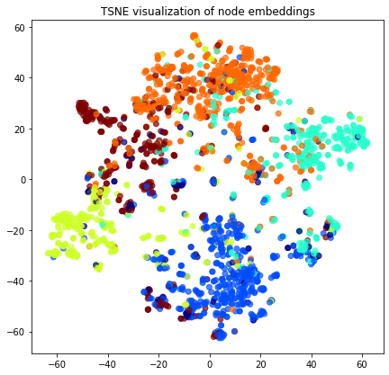
Transform the embeddings to 2d space for visualisation.
[17]:
transform = TSNE  # PCA

trans = transform(n_components=2)
node_embeddings_2d = trans.fit_transform(node_embeddings)
[18]:
# draw the embedding points, coloring them by the target label (paper subject)
alpha = 0.7
label_map = {l: i for i, l in enumerate(np.unique(subjects))}
node_colours = [label_map[target] for target in subjects]

plt.figure(figsize=(7, 7))
plt.axes().set(aspect="equal")
plt.scatter(
    node_embeddings_2d[:, 0],
    node_embeddings_2d[:, 1],
    c=node_colours,
    cmap="jet",
    alpha=alpha,
)
plt.title("{} visualization of node embeddings".format(transform.__name__))
plt.show()
Node Classificaion Task
The embeddings learned by attri2vec can be used as feature vectors in downstream tasks, such as node classification and link prediction.
In this example, we will use the attri2vec node embeddings to train a classifier to predict the subject of a paper in DBLP.
[19]:
# X will hold the 128-dimensional input features
X = node_embeddings
# y holds the corresponding target values
y = np.array(subjects)
Data Splitting
We split the data into train and test sets.
We use 20% of the data for training and the remaining 80% for testing as a hold out test set.
[20]:
X_train, X_test, y_train, y_test = train_test_split(X, y, train_size=0.2, test_size=None)
print(
    "Array shapes:\n X_train = {}\n y_train = {}\n X_test = {}\n y_test = {}".format(
        X_train.shape, y_train.shape, X_test.shape, y_test.shape
    )
)
Array shapes:
 X_train = (422, 128)
 y_train = (422,)
 X_test = (1688, 128)
 y_test = (1688,)
Classifier Training
We train a Logistic Regression classifier on the training data.
[21]:
clf = LogisticRegressionCV(
    Cs=10, cv=10, scoring="accuracy", verbose=False, multi_class="ovr", max_iter=1000
)
clf.fit(X_train, y_train)
[21]:
LogisticRegressionCV(Cs=10, class_weight=None, cv=10, dual=False,
                     fit_intercept=True, intercept_scaling=1.0, l1_ratios=None,
                     max_iter=1000, multi_class='ovr', n_jobs=None,
                     penalty='l2', random_state=None, refit=True,
                     scoring='accuracy', solver='lbfgs', tol=0.0001,
                     verbose=False)
Predict the hold-out test set.
[22]:
y_pred = clf.predict(X_test)
Calculate the accuracy of the classifier on the test set.
[23]:
accuracy_score(y_test, y_pred)
[23]:
0.754739336492891
Run the master version of this notebook: |