Stellargraph example: Heterogeneous GraphSAGE on the Movielens recommendation dataset
Run the master version of this notebook: |
In this example, we use our generalisation of the GraphSAGE algorithm to heterogeneous graphs (which we call HinSAGE) to build a model that predicts user-movie ratings in the Movielens dataset (see below). The problem is treated as a supervised link attribute inference problem on a user-movie network with nodes of two types (users and movies, both attributed) and links corresponding to user-movie ratings, with integer rating attributes from 1 to 5
(note that if a user hasn’t rated a movie, the corresponding user-movie link does not exist in the network).
To address this problem, we build a model with the following architecture: a two-layer HinSAGE model that takes labeled (user, movie) node pairs corresponding to user-movie ratings, and outputs a pair of node embeddings for the user and movie nodes of the pair. These embeddings are then fed into a link regression layer, which applies a binary operator to those node embeddings (e.g., concatenating them) to construct the link embedding. Thus obtained link embeddings are passed through
the link regression layer to obtain predicted user-movie ratings. The entire model is trained end-to-end by minimizing the loss function of choice (e.g., root mean square error between predicted and true ratings) using stochastic gradient descent (SGD) updates of the model parameters, with minibatches of user-movie training links fed into the model.
[1]:
# install StellarGraph if running on Google Colab
import sys
if 'google.colab' in sys.modules:
  %pip install -q stellargraph[demos]==1.0.0rc1
[2]:
# verify that we're using the correct version of StellarGraph for this notebook
import stellargraph as sg

try:
    sg.utils.validate_notebook_version("1.0.0rc1")
except AttributeError:
    raise ValueError(
        f"This notebook requires StellarGraph version 1.0.0rc1, but a different version {sg.__version__} is installed.  Please see <https://github.com/stellargraph/stellargraph/issues/1172>."
    ) from None
[3]:
import json
import pandas as pd
import numpy as np
from sklearn import preprocessing, feature_extraction, model_selection
from sklearn.metrics import mean_absolute_error, mean_squared_error

import stellargraph as sg
from stellargraph.mapper import HinSAGELinkGenerator
from stellargraph.layer import HinSAGE, link_regression
from tensorflow.keras import Model, optimizers, losses, metrics

import multiprocessing
from stellargraph import datasets
from IPython.display import display, HTML
import matplotlib.pyplot as plt
%matplotlib inline
Specify the minibatch size (number of user-movie links per minibatch) and the number of epochs for training the ML model:
[4]:
batch_size = 200
epochs = 20
# Use 70% of edges for training, the rest for testing:
train_size = 0.7
test_size = 0.3
Load the dataset
[5]:
dataset = datasets.MovieLens()
display(HTML(dataset.description))
G, edges_with_ratings = dataset.load()
[6]:
print(G.info())
StellarGraph: Undirected multigraph
 Nodes: 2625, Edges: 100000

 Node types:
  movie: [1682]
    Features: float32 vector, length 19
    Edge types: movie-rating->user
  user: [943]
    Features: float32 vector, length 24
    Edge types: user-rating->movie

 Edge types:
    user-rating->movie: [100000]
Split the edges into train and test sets for model training/evaluation:
[7]:
edges_train, edges_test = model_selection.train_test_split(
    edges_with_ratings, train_size=train_size, test_size=test_size
)

edgelist_train = list(edges_train[["user_id", "movie_id"]].itertuples(index=False))
edgelist_test = list(edges_test[["user_id", "movie_id"]].itertuples(index=False))

labels_train = edges_train["rating"]
labels_test = edges_test["rating"]
Our machine learning task of learning user-movie ratings can be framed as a supervised Link Attribute Inference: given a graph of user-movie ratings, we train a model for rating prediction using the ratings edges_train, and evaluate it using the test ratings edges_test. The model also requires the user-movie graph structure, to do the neighbour sampling required by the HinSAGE algorithm.
We create the link mappers for sampling and streaming training and testing data to the model. The link mappers essentially “map” user-movie links to the input of HinSAGE: they take minibatches of user-movie links, sample 2-hop subgraphs of G with (user, movie) head nodes extracted from those user-movie links, and feed them, together with the corresponding user-movie ratings, to the input layer of the HinSAGE model, for SGD updates of the model parameters.
Specify the sizes of 1- and 2-hop neighbour samples for HinSAGE:
Note that the length of num_samples list defines the number of layers/iterations in the HinSAGE model.
[8]:
num_samples = [8, 4]
Create the generators to feed data from the graph to the Keras model. We need to specify the nodes types for the user-movie pairs that we will feed to the model. The shuffle=True argument is given to the flow method to improve training.
[9]:
generator = HinSAGELinkGenerator(
    G, batch_size, num_samples, head_node_types=["user", "movie"]
)
train_gen = generator.flow(edgelist_train, labels_train, shuffle=True)
test_gen = generator.flow(edgelist_test, labels_test)
Build the model by stacking a two-layer HinSAGE model and a link regression layer on top.
First, we define the HinSAGE part of the model, with hidden layer sizes of 32 for both HinSAGE layers, a bias term, and no dropout. (Dropout can be switched on by specifying a positive dropout rate, 0 < dropout < 1)
Note that the length of layer_sizes list must be equal to the length of num_samples, as len(num_samples) defines the number of hops (layers) in the HinSAGE model.
[10]:
generator.schema.type_adjacency_list(generator.head_node_types, len(num_samples))
[10]:
[('user', [2]),
 ('movie', [3]),
 ('movie', [4]),
 ('user', [5]),
 ('user', []),
 ('movie', [])]
[11]:
generator.schema.schema
[11]:
{'user': [EdgeType(n1='user', rel='rating', n2='movie')],
 'movie': [EdgeType(n1='movie', rel='rating', n2='user')]}
[12]:
hinsage_layer_sizes = [32, 32]
assert len(hinsage_layer_sizes) == len(num_samples)

hinsage = HinSAGE(
    layer_sizes=hinsage_layer_sizes, generator=generator, bias=True, dropout=0.0
)
[13]:
# Expose input and output sockets of hinsage:
x_inp, x_out = hinsage.in_out_tensors()
Add the final estimator layer for predicting the ratings. The edge_embedding_method argument specifies the way in which node representations (node embeddings) are combined into link representations (recall that links represent user-movie ratings, and are thus pairs of (user, movie) nodes). In this example, we will use ‘concat’, i.e., node embeddings are concatenated to get link embeddings.
[14]:
# Final estimator layer
score_prediction = link_regression(edge_embedding_method="concat")(x_out)
link_regression: using 'concat' method to combine node embeddings into edge embeddings
Create the Keras model, and compile it by specifying the optimizer, loss function to optimise, and metrics for diagnostics:
[15]:
import tensorflow.keras.backend as K


def root_mean_square_error(s_true, s_pred):
    return K.sqrt(K.mean(K.pow(s_true - s_pred, 2)))


model = Model(inputs=x_inp, outputs=score_prediction)
model.compile(
    optimizer=optimizers.Adam(lr=1e-2),
    loss=losses.mean_squared_error,
    metrics=[root_mean_square_error, metrics.mae],
)
Summary of the model:
[16]:
model.summary()
Model: "model"
__________________________________________________________________________________________________
Layer (type)                    Output Shape         Param #     Connected to
==================================================================================================
input_3 (InputLayer)            [(None, 8, 19)]      0
__________________________________________________________________________________________________
input_5 (InputLayer)            [(None, 32, 24)]     0
__________________________________________________________________________________________________
input_6 (InputLayer)            [(None, 32, 19)]     0
__________________________________________________________________________________________________
input_1 (InputLayer)            [(None, 1, 24)]      0
__________________________________________________________________________________________________
reshape (Reshape)               (None, 1, 8, 19)     0           input_3[0][0]
__________________________________________________________________________________________________
reshape_2 (Reshape)             (None, 8, 4, 24)     0           input_5[0][0]
__________________________________________________________________________________________________
input_4 (InputLayer)            [(None, 8, 24)]      0
__________________________________________________________________________________________________
reshape_3 (Reshape)             (None, 8, 4, 19)     0           input_6[0][0]
__________________________________________________________________________________________________
dropout_1 (Dropout)             (None, 1, 24)        0           input_1[0][0]
__________________________________________________________________________________________________
dropout (Dropout)               (None, 1, 8, 19)     0           reshape[0][0]
__________________________________________________________________________________________________
dropout_5 (Dropout)             (None, 8, 19)        0           input_3[0][0]
__________________________________________________________________________________________________
dropout_4 (Dropout)             (None, 8, 4, 24)     0           reshape_2[0][0]
__________________________________________________________________________________________________
input_2 (InputLayer)            [(None, 1, 19)]      0
__________________________________________________________________________________________________
reshape_1 (Reshape)             (None, 1, 8, 24)     0           input_4[0][0]
__________________________________________________________________________________________________
dropout_7 (Dropout)             (None, 8, 24)        0           input_4[0][0]
__________________________________________________________________________________________________
dropout_6 (Dropout)             (None, 8, 4, 19)     0           reshape_3[0][0]
__________________________________________________________________________________________________
mean_hin_aggregator (MeanHinAgg multiple             720         dropout_1[0][0]
                                                                 dropout[0][0]
                                                                 dropout_7[0][0]
                                                                 dropout_6[0][0]
__________________________________________________________________________________________________
mean_hin_aggregator_1 (MeanHinA multiple             720         dropout_3[0][0]
                                                                 dropout_2[0][0]
                                                                 dropout_5[0][0]
                                                                 dropout_4[0][0]
__________________________________________________________________________________________________
dropout_3 (Dropout)             (None, 1, 19)        0           input_2[0][0]
__________________________________________________________________________________________________
dropout_2 (Dropout)             (None, 1, 8, 24)     0           reshape_1[0][0]
__________________________________________________________________________________________________
reshape_4 (Reshape)             (None, 1, 8, 32)     0           mean_hin_aggregator_1[1][0]
__________________________________________________________________________________________________
reshape_5 (Reshape)             (None, 1, 8, 32)     0           mean_hin_aggregator[1][0]
__________________________________________________________________________________________________
dropout_9 (Dropout)             (None, 1, 32)        0           mean_hin_aggregator[0][0]
__________________________________________________________________________________________________
dropout_8 (Dropout)             (None, 1, 8, 32)     0           reshape_4[0][0]
__________________________________________________________________________________________________
dropout_11 (Dropout)            (None, 1, 32)        0           mean_hin_aggregator_1[0][0]
__________________________________________________________________________________________________
dropout_10 (Dropout)            (None, 1, 8, 32)     0           reshape_5[0][0]
__________________________________________________________________________________________________
mean_hin_aggregator_2 (MeanHinA (None, 1, 32)        1056        dropout_9[0][0]
                                                                 dropout_8[0][0]
__________________________________________________________________________________________________
mean_hin_aggregator_3 (MeanHinA (None, 1, 32)        1056        dropout_11[0][0]
                                                                 dropout_10[0][0]
__________________________________________________________________________________________________
reshape_6 (Reshape)             (None, 32)           0           mean_hin_aggregator_2[0][0]
__________________________________________________________________________________________________
reshape_7 (Reshape)             (None, 32)           0           mean_hin_aggregator_3[0][0]
__________________________________________________________________________________________________
lambda (Lambda)                 (None, 32)           0           reshape_6[0][0]
                                                                 reshape_7[0][0]
__________________________________________________________________________________________________
link_embedding (LinkEmbedding)  (None, 64)           0           lambda[0][0]
                                                                 lambda[1][0]
__________________________________________________________________________________________________
dense (Dense)                   (None, 1)            65          link_embedding[0][0]
__________________________________________________________________________________________________
reshape_8 (Reshape)             (None, 1)            0           dense[0][0]
==================================================================================================
Total params: 3,617
Trainable params: 3,617
Non-trainable params: 0
__________________________________________________________________________________________________
[17]:
# Specify the number of workers to use for model training
num_workers = 4
Evaluate the fresh (untrained) model on the test set (for reference):
[18]:
test_metrics = model.evaluate(
    test_gen, verbose=1, use_multiprocessing=False, workers=num_workers
)

print("Untrained model's Test Evaluation:")
for name, val in zip(model.metrics_names, test_metrics):
    print("\t{}: {:0.4f}".format(name, val))
  ['...']
150/150 [==============================] - 25s 165ms/step - loss: 11.8834 - root_mean_square_error: 3.4467 - mean_absolute_error: 3.256210s - loss: 11.8462 - root_mean_square_erro
Untrained model's Test Evaluation:
        loss: 11.8834
        root_mean_square_error: 3.4467
        mean_absolute_error: 3.2562
Train the model by feeding the data from the graph in minibatches, using mapper_train, and get validation metrics after each epoch:
[19]:
history = model.fit(
    train_gen,
    validation_data=test_gen,
    epochs=epochs,
    verbose=1,
    shuffle=False,
    use_multiprocessing=False,
    workers=num_workers,
)
  ['...']
  ['...']
Train for 350 steps, validate for 150 steps
Epoch 1/20
350/350 [==============================] - 87s 249ms/step - loss: 1.3311 - root_mean_square_error: 1.1321 - mean_absolute_error: 0.9363 - val_loss: 1.1607 - val_root_mean_square_error: 1.0759 - val_mean_absolute_error: 0.8687error: 1.13
Epoch 2/20
350/350 [==============================] - 85s 244ms/step - loss: 1.1525 - root_mean_square_error: 1.0724 - mean_absolute_error: 0.8711 - val_loss: 1.1315 - val_root_mean_square_error: 1.0624 - val_mean_absolute_error: 0.8693s -  - ETA: 2
Epoch 3/20
350/350 [==============================] - 90s 256ms/step - loss: 1.1357 - root_mean_square_error: 1.0645 - mean_absolute_error: 0.8626 - val_loss: 1.1141 - val_root_mean_square_error: 1.0542 - val_mean_absolute_error: 0.8612 loss: 1.1321 - root_mean_square_error: 1.0628 - mean_absolute_error: - ETA: 10s - loss:
Epoch 4/20
350/350 [==============================] - 83s 236ms/step - loss: 1.1235 - root_mean_square_error: 1.0588 - mean_absolute_error: 0.8566 - val_loss: 1.1035 - val_root_mean_square_error: 1.0489 - val_mean_absolute_error: 0.8432
Epoch 5/20
350/350 [==============================] - 89s 255ms/step - loss: 1.1148 - root_mean_square_error: 1.0546 - mean_absolute_error: 0.8526 - val_loss: 1.1057 - val_root_mean_square_error: 1.0500 - val_mean_absolute_error: 0.8372are_error: 1.05 - ETA: 21s - loss: 1.1116 - root_mean_square_error: 1.0531 - mean_abso - E - ETA: 4s - loss: 1.1130 - root_mean_square_error: 1.0537 - mean_abso
Epoch 6/20
350/350 [==============================] - 85s 243ms/step - loss: 1.1123 - root_mean_square_error: 1.0533 - mean_absolute_error: 0.8517 - val_loss: 1.0983 - val_root_mean_square_error: 1.0466 - val_mean_absolute_error: 0.8461
Epoch 7/20
350/350 [==============================] - 100s 286ms/step - loss: 1.1096 - root_mean_square_error: 1.0523 - mean_absolute_error: 0.8498 - val_loss: 1.0966 - val_root_mean_square_error: 1.0458 - val_mean_absolute_error: 0.8538ot_me - ETA: 39s - loss: 1.1068 - root_mean_square_error: 1.0510 - mean_absolu - E - ETA: 18s - loss: 1.1056 - root_mean_square_error: 1.0504 - mean_absolu - ETA: 14s - loss: 1.1078 - ETA: 6s - loss: 1.1085 - root_mean_square_e
Epoch 8/20
350/350 [==============================] - 91s 261ms/step - loss: 1.1049 - root_mean_square_error: 1.0502 - mean_absolute_error: 0.8478 - val_loss: 1.0947 - val_root_mean_square_error: 1.0449 - val_mean_absolute_error: 0.8489 1:44 - loss: 1.0948 - root_mean_square_error: 1.0454 - mean_absolute_error: 0. - ETA: 1:42 - loss: 1.0966 - root_mean_square_error: 1.04 - ETA: 1:32 - loss: 1.0876 - root_mean_square_error: 1.0419 - mean_absolute_error - ETA: 1:30 - loss: 1.0922 - root_mean_square_error: 1.04 - ETA: 1:19 - loss: 1.0931 - root_mean_squa - ETA: 1:05 - loss: 1.0975 - root_mean_square_error: 1. - ETA: 54s - loss: 1.0982 - root_mean_square_error - ETA: 40s - loss: 1.1085 - root_mean_square_e - ETA: 27s - loss: 1.1068 - root_mean_square_error: 1.0511 - mean_absolute_error:  - ETA: 25s - loss: 1.1083 - root - ETA: 12s - loss:
Epoch 9/20
350/350 [==============================] - 79s 225ms/step - loss: 1.1031 - root_mean_square_error: 1.0490 - mean_absolute_error: 0.8473 - val_loss: 1.0926 - val_root_mean_square_error: 1.0439 - val_mean_absolute_error: 0.8503
Epoch 10/20
350/350 [==============================] - 79s 225ms/step - loss: 1.0967 - root_mean_square_error: 1.0461 - mean_absolute_error: 0.8439 - val_loss: 1.0842 - val_root_mean_square_error: 1.0399 - val_mean_absolute_error: 0.8402root_mean_squa - ETA: 28s - loss: 1.0982 - root_mean_square_error: 1.0467 - mean_absolute_err - ETA: 26s - loss: 1  - ETA: 3s - loss: 1.0969 - root_mean_square_error: 1.0461 - mean_absolu
Epoch 11/20
350/350 [==============================] - 79s 226ms/step - loss: 1.0955 - root_mean_square_error: 1.0455 - mean_absolute_error: 0.8437 - val_loss: 1.0832 - val_root_mean_square_error: 1.0394 - val_mean_absolute_error: 0.8402
Epoch 12/20
350/350 [==============================] - 104s 298ms/step - loss: 1.0948 - root_mean_square_error: 1.0453 - mean_absolute_error: 0.8426 - val_loss: 1.0866 - val_root_mean_square_error: 1.0411 - val_mean_absolute_error: 0.8448square_error: 1.0466 - m - ETA: 6s - loss: 1.0970 - root_mean_square_error: 1.0463 - mean_ - ETA: 4s - loss: 1.0953 - root_mean_square_error: 1.0455 - mean_absolu
Epoch 13/20
350/350 [==============================] - 132s 377ms/step - loss: 1.0941 - root_mean_square_error: 1.0448 - mean_absolute_error: 0.8431 - val_loss: 1.0867 - val_root_mean_square_error: 1.0410 - val_mean_absolute_error: 0.8492 loss: 1.0591 - root_mean_square_error: 1.0280 - mean_absolute_error:  - ETA: 3:08 - loss: 1.0806 - root_mean_square_error: 1.0383 - mean_absolu - ETA: 2:31 - loss: 1.0934 - root_mean_square_error: 1.0448 - mean_absolute_error:  - ETA: 2:22 - loss: 1.093 - ETA: 1:38 - loss: 1.0824 - root_mean_square_error: 1.03 - ETA: 1:27 - loss: 1.0839 - root_mean_square_error: 1.0401 - ETA: 1:20 - loss: 1.0836 - root_mean_square_error - ETA: 51s - loss: 1.0905 - root_mean_square_error: 1.0432 - me - ETA: 44s - loss: 1.0910 - root_mean_square_error: 1.0433 - mean_absolute_error: 0. - ETA: 42s - loss: 1.0926 - root_mean_squa - ETA: 29s - loss: 1.0936 - root_mean_square_error: 1.0445 - mean - ETA: 22s - loss: 1.0910 - root_mean_square_error: 1.0433 - mean_absolute_error: 0.842 - ETA: 22s - loss: 1.0905 - root_mean_square_error: 1.0430 - mean_absolute_error:  - ETA: 20s - loss: 1.0901 - root_mean_square_error: 1.0429 - mean_absolute_error: 0. - ETA: 19s - loss: 1.0899 - root_mean_square_error: 1 - ETA: 9s - loss: 1.0915 - root_mean_square_
Epoch 14/20
350/350 [==============================] - 109s 311ms/step - loss: 1.0895 - root_mean_square_error: 1.0426 - mean_absolute_error: 0.8408 - val_loss: 1.0872 - val_root_mean_square_error: 1.0411 - val_mean_absolute_error: 0.8332square_error:  - ETA: 1:02 - loss: 1.0780 - root_mean_square_error: 1.0371 - mean_absolute_error: 0. - ETA: 1:02 - loss: 1.0764 - root_mean_square_error: 1.0364 - mean_a - ETA: 58s - loss: 1.0809 - root_mean_square_error: 1.0386 - mean_abso - ETA: 53s - loss: 1.0807 - root_mean_square_error: 1.0384 - m - ETA: 46s - loss: 1.0810 - r - ETA: 26s - loss: 1.0835 - root_mean_square_ - ETA: 14s - loss: 1.0863 - root_mean_square_error: 1.0410 - mean_absolute_error: 0 - ETA: 13s -
Epoch 15/20
350/350 [==============================] - 100s 286ms/step - loss: 1.0880 - root_mean_square_error: 1.0419 - mean_absolute_error: 0.8412 - val_loss: 1.0884 - val_root_mean_square_error: 1.0418 - val_mean_absolute_error: 0.8358absolute_error: 0.84 - ETA: 28s - loss: 1.0879 - root_mean_square_error: 1.0419 - mean_absolute_error: 0.84 - ETA: 28s - loss: 1.0876 -  - ETA: 11s - loss: 1.0885 - root_mean_square_error: 1.0421 - mean_absolute_error: 0.8 - ETA: 11s - loss: 1.0877 - root_mean_square_error: 1.0417 - mean_absol - ETA: 8s - loss: 1.0888 - root_mean_square_err
Epoch 16/20
350/350 [==============================] - 82s 234ms/step - loss: 1.0857 - root_mean_square_error: 1.0409 - mean_absolute_error: 0.8401 - val_loss: 1.0833 - val_root_mean_square_error: 1.0392 - val_mean_absolute_error: 0.8332
Epoch 17/20
350/350 [==============================] - 87s 247ms/step - loss: 1.0837 - root_mean_square_error: 1.0398 - mean_absolute_error: 0.8387 - val_loss: 1.0744 - val_root_mean_square_error: 1.0351 - val_mean_absolute_error: 0.8348
Epoch 18/20
350/350 [==============================] - 88s 251ms/step - loss: 1.0840 - root_mean_square_error: 1.0400 - mean_absolute_error: 0.8389 - val_loss: 1.0878 - val_root_mean_square_error: 1.0416 - val_mean_absolute_error: 0.8527_square_error: 1.0385 - mean_absolute_erro - ETA: 17s - - ETA: 5s - loss: 1.0813 - root_mean_square_error: 1.0387 -
Epoch 19/20
350/350 [==============================] - 83s 236ms/step - loss: 1.0798 - root_mean_square_error: 1.0380 - mean_absolute_error: 0.8371 - val_loss: 1.0728 - val_root_mean_square_error: 1.0344 - val_mean_absolute_error: 0.8424
Epoch 20/20
350/350 [==============================] - 79s 227ms/step - loss: 1.0815 - root_mean_square_error: 1.0386 - mean_absolute_error: 0.8387 - val_loss: 1.0680 - val_root_mean_square_error: 1.0319 - val_mean_absolute_error: 0.83024s - loss: 1.0764 - root_mean_square_error: 1.0362 - me - ETA: 38s - loss: 1.0777 - root_
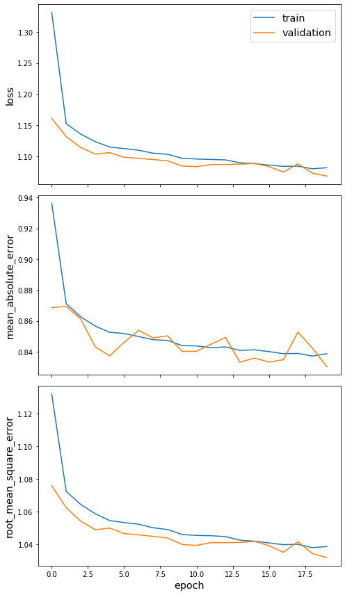
Plot the training history:
[20]:
sg.utils.plot_history(history)
Evaluate the trained model on test user-movie rankings:
[21]:
test_metrics = model.evaluate(
    test_gen, use_multiprocessing=False, workers=num_workers, verbose=1
)

print("Test Evaluation:")
for name, val in zip(model.metrics_names, test_metrics):
    print("\t{}: {:0.4f}".format(name, val))
  ['...']
150/150 [==============================] - 23s 152ms/step - loss: 1.0738 - root_mean_square_error: 1.0347 - mean_absolute_error: 0.8325 44s - loss: 1.0911 - root_mean_square
Test Evaluation:
        loss: 1.0738
        root_mean_square_error: 1.0347
        mean_absolute_error: 0.8325
Compare the predicted test rankings with “mean baseline” rankings, to see how much better our model does compared to this (very simplistic) baseline:
[22]:
y_true = labels_test
# Predict the rankings using the model:
y_pred = model.predict(test_gen)
# Mean baseline rankings = mean movie ranking:
y_pred_baseline = np.full_like(y_pred, np.mean(y_true))

rmse = np.sqrt(mean_squared_error(y_true, y_pred_baseline))
mae = mean_absolute_error(y_true, y_pred_baseline)
print("Mean Baseline Test set metrics:")
print("\troot_mean_square_error = ", rmse)
print("\tmean_absolute_error = ", mae)

rmse = np.sqrt(mean_squared_error(y_true, y_pred))
mae = mean_absolute_error(y_true, y_pred)
print("\nModel Test set metrics:")
print("\troot_mean_square_error = ", rmse)
print("\tmean_absolute_error = ", mae)
Mean Baseline Test set metrics:
        root_mean_square_error =  1.1250835578845824
        mean_absolute_error =  0.9442556604067485

Model Test set metrics:
        root_mean_square_error =  1.0363648722884464
        mean_absolute_error =  0.8332940764943758
Compare the distributions of predicted and true rankings for the test set:
[23]:
h_true = plt.hist(y_true, bins=30, facecolor="green", alpha=0.5)
h_pred = plt.hist(y_pred, bins=30, facecolor="blue", alpha=0.5)
plt.xlabel("ranking")
plt.ylabel("count")
plt.legend(("True", "Predicted"))
plt.show()
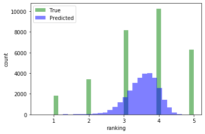
We see that our model beats the “mean baseline” by a significant margin. To further improve the model, you can try increasing the number of training epochs, change the dropout rate, change the sample sizes for subgraph sampling num_samples, hidden layer sizes layer_sizes of the HinSAGE part of the model, or try increasing the number of HinSAGE layers.
However, note that the distribution of predicted scores is still very narrow, and rarely gives 1, 2 or 5 as a score.
This model uses a bipartite user-movie graph to learn to predict movie ratings. It can be further enhanced by using additional relations, e.g., friendships between users, if they become available. And the best part is: the underlying algorithm of the model does not need to change at all to take these extra relations into account - all that changes is the graph that it learns from!
Run the master version of this notebook: |